View allAll Photos Tagged random_variation
Up close and personal with one of our larger shorebirds. I made this shot last spring from the rolling red Toyota blind. On foot, I could never get this close to one, like I did for yesterday's American White Pelican. Of course, the pelican is a much larger bird, and I was able to fill the frame from a greater distance. The excitement of wildlife photography is due in great measure to its unpredictability: every situation is different. You have to work with pre-existing backgrounds, random variations in quality of light, unpredictable behaviour, varying degrees of proximity, bad weather, physical exertion, chance encounters that are often very brief, long periods of nothing happening punctuated by flurries of action, and lots of disappointment. And through all this... the adventure and the satisfaction of coming home with good stuff in the bag. It isn't for everyone; it takes a special breed. That's us.
Photographed at Reed Lake, Saskatchewan (Canada). Don't use this image on websites, blogs, or other media without explicit permission ©2020 James R. Page - all rights reserved.
I’d call this a “stellar” snowflake, which is relatively rare. Usually you’d find side-branches filling in the shape to a greater degree, and running along the main branches is a colourful surprise. You need to take a closer look and view large!
The center of this snowflake reveals a different past. The three-fold symmetry is beautiful and indicates a more “triangular” beginning. Things even out as the branches reach farther away from the center, where random variations average out any initial pattern created by the aerodynamic properties of the snowflake. I love seeing these shapes – they reveal a curious beauty by breaking full symmetry, but creating another kind.
The branches reveal a beautiful feature of crystals of any kind: a “prism” effect. Rainbows and colour in snow are caused by two primary phenomenon: thin film interference, and simple splitting of light the way a prism does. Certain features of a snowflake can split light into its component wavelengths, resulting in rainbows of colour being generated inside the branches. The rainbow doesn’t appear in the proper order as one might expect, colours might shift unexpectedly and certain colours might be more prevalent based on the growth pattern of the crystal.
Some of the colour, mostly subtle magentas and cyans are created by colour fringing. In some cases there is evidence that this occurs in the crystal, other evidence points towards the camera lens. For colours that seem clearly created by the camera equipment, I try to subdue them while allowing the natural colour in the snowflake to stay saturated. Careful attention to colour is given to every snowflake, even the ones without any noticeable colour phenomenon. I endeavour to make them as “real” as possible!
The rounded branch tips are a sign that this snowflake has already started to disappear. There aren’t any signs of melting, so we’re left to conclude that this snowflake has already begun evaporating. This process begins as soon as the snowflake leaves the cloud that created it, and continues until it is nothing more than a blob of ice. Such a fleeting existence makes these tiny crystals all the more beautiful.
For more snowflake physics including many pages dedicated to the colour of snow, check out Sky Crystals: skycrystals.ca/book/ - walk through every type of snowflake and understand how they’re all formed, and learn every technique required to photograph them and explore winter’s beauty for yourself.
To see what all of my time with the subject of snowflakes looks in a single image, check out “The Snowflake” print: skycrystals.ca/poster/ - I’m proud to say that I doubt anyone else will ever attempt to create anything like it. :)
Looking like a glittering cosmic geode, a trio of dazzling stars blaze from the hollowed-out cavity of a reflection nebula in this new image from NASA’s Hubble Space Telescope. The triple-star system is made up of the variable star HP Tau, HP Tau G2, and HP Tau G3. HP Tau is known as a T Tauri star, a type of young variable star that hasn’t begun nuclear fusion yet but is beginning to evolve into a hydrogen-fueled star similar to our Sun. T Tauri stars tend to be younger than 10 million years old - in comparison, our Sun is around 4.6 billion years old - and are often found still swaddled in the clouds of dust and gas from which they formed.
As with all variable stars, HP Tau’s brightness changes over time. T Tauri stars are known to have both periodic and random fluctuations in brightness. The random variations may be due to the chaotic nature of a developing young star, such as instabilities in the accretion disk of dust and gas around the star, material from that disk falling onto the star and being consumed, and flares on the star’s surface. The periodic changes may be due to giant sunspots rotating in and out of view.
Credit: NASA, ESA, G. Duchene (Universite de Grenoble I); Image Processing: Gladys Kober (NASA/Catholic University of America)
#NASA #NASAGoddard #NASAMarshall #NASAGoddard #HubbleSpaceTelescope #HST #ESA #nebula #star
In an effort to show the unlimited complexities of snowflakes, here is a simple star design, a common type of snowflake that falls by the trillions every year, but with a unique twist – colour in the center with a pattern that cannot be replicated exactly, ever again. Every snowflake is unique! View Large! (press the "L" key to turn on Lightbox mode!)
Snowflakes are complex creations. Governed by a few simple set of physics “rules”, add in the number of molecules required (many quintillion) and pseudo-random variations in temperature, humidity, wind speed, etc. and you’ve got a recipe for unique structures every time. No two snowflakes are ever alike. Some might look similar on the surface, but details reveal another story… and I’m glad I can showcase the details within this series. :)
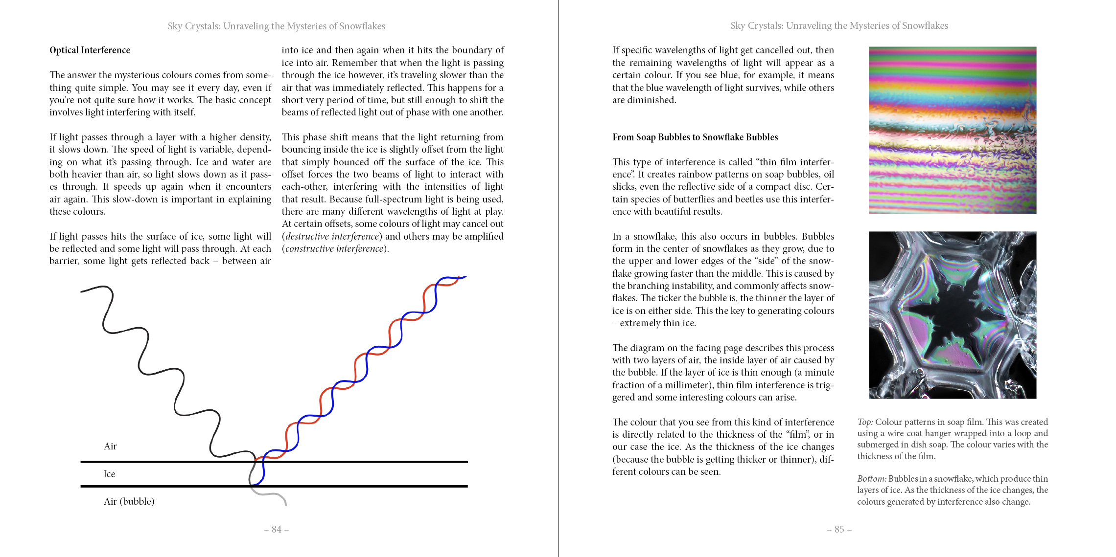
The colour, for example, is produced by multiple layers of air and ice that evoke the phenomenon known as “thin film interference”. For those that have read these descriptions before, I’ll stop myself from sounding like a broken record. For those curious what the heck “thin film interference”, check out these pages of Sky Crystals for a very good explanation: skycrystals.ca/pages/optical-interference-pages.jpg
The patterns of colour are determined by the thickness of ice and air, and as these two variables change, so too does the resulting colour. The inner part of this snowflake has a “shield”, a top plate layer which is part of a fully-grown “capped column” crystal that might be contributing to this effect… but it only echoes the same idea: these are incredibly small, but incredibly complex things. Measuring roughly 1.5mm in diameter, this snowflake and trillions like it go completely unnoticed every year, but the result is the same in each one: untold complexity that results in untold beauty.
Of course, photographing these snowflakes can be quite difficult. Earlier this evening I was fortunate enough to be featured on another episode of the Jpeg2Raw video podcast and while I featured a fair amount of my work, this snowflakes was used as an example for my editing workflow. I’ll post a link to that episode when it goes live. And you’ll see what is involved in producing this final image. About three and a half hours were dedicated to this crystal, even though (only!) 24 layers were used in the focus stacking part of the process. Plenty of effort is placed into each image, in order to create a scientifically accurate and photographically beautiful image. Rarely do those two things run hand-in-hand!
This entire series of images is based on my love for science, and my love for photography. Snowflakes are perfect subject to bridge that gap, but my personal enjoyment isn’t enough. I wanted to share the experience of discovery with everyone, so I wrote and published a book called Sky Crystals: www.skycrystals.ca/ which details all of the science (in an easy-to-understand way) with all of the photographic techniques in exhaustive detail. Check it out if you have a love of nature, physics and photography like myself. Or check it out if you simply enjoy these images. :)
The nature versus nurture debate concerns the relative importance of an individual's innate qualities ("nature," i.e. nativism, or innatism) versus personal experiences ("nurture," i.e. empiricism or behaviorism) in determining or causing individual differences in physical and behavioral traits.
"Nature versus nurture" in its modern sense was coined by the English Victorian polymath Francis Galton in discussion of the influence of heredity and environment on social advancement, although the terms had been contrasted previously, for example by Shakespeare (The Tempest). Galton was influenced by the book On the Origin of Species written by his cousin, Charles Darwin. The concept embodied in the phrase has been criticized for its binary simplification of two tightly interwoven parameters, as for example an environment of wealth, education and social privilege are often historically passed to genetic offspring.
The view that humans acquire all or almost all their behavioral traits from "nurture" is known as tabula rasa ("blank slate"). This question was once considered to be an appropriate division of developmental influences, but since both types of factors are known to play such interacting roles in development, many modern psychologists consider the question naive—representing an outdated state of knowledge. Psychologist Donald Hebb is said to have once answered a journalist's question of "which, nature or nurture, contributes more to personality?" by asking in response, "Which contributes more to the area of a rectangle, its length or its width?" That is, the idea that either nature or nurture explains a creature's behavior is a sort of single cause fallacy.
In the social and political sciences, the nature versus nurture debate may be contrasted with the structure versus agency debate (i.e. socialization versus individual autonomy). For a discussion of nature versus nurture in language and other human universals, see also psychological nativism.
Personality is a frequently cited example of a heritable trait that has been studied in twins and adoptions. Identical twins reared apart are far more similar in personality than randomly selected pairs of people. Likewise, identical twins are more similar than fraternal twins. Also, biological siblings are more similar in personality than adoptive siblings. Each observation suggests that personality is heritable to a certain extent. However, these same study designs allow for the examination of environment as well as genes. Adoption studies also directly measure the strength of shared family effects. Adopted siblings share only family environment. Unexpectedly, some adoption studies indicate that by adulthood the personalities of adopted siblings are no more similar than random pairs of strangers. This would mean that shared family effects on personality are zero by adulthood. As is the case with personality, non-shared environmental effects are often found to out-weigh shared environmental effects. That is, environmental effects that are typically thought to be life-shaping (such as family life) may have less of an impact than non-shared effects, which are harder to identify. One possible source of non-shared effects is the environment of pre-natal development. Random variations in the genetic program of development may be a substantial source of non-shared environment. These results suggest that "nurture" may not be the predominant factor in "environment."
The speckled wood (Pararge aegeria) is a butterfly found in and on the borders of woodland areas throughout much of the Palearctic realm. The species is subdivided into multiple subspecies, including Pararge aegeria aegeria, Pararge aegeria tircis, Pararge aegeria oblita, and Pararge aegeria insula. The color of this butterfly varies between subspecies. The existence of these subspecies is due to variation in morphology down a gradient corresponding to a geographic cline. The background of the wings ranges from brown to orange, and the spots are either pale yellow, white, cream, or a tawny orange. The speckled wood feeds on a variety of grass species. The males of this species exhibit two types of mate locating behaviors: territorial defense and patrolling. The proportion of males exhibiting these two strategies changes based on ecological conditions. The monandrous female must choose which type of male can help her reproduce successfully. Her decision is heavily influenced by environmental conditions.
Taxonomy
The speckled wood belongs to the genus Pararge, which comprises three species: Pararge aegeria, Pararge xiphia, and Pararge xiphioides. Pararge xiphia occurs on the Atlantic island of Madeira. Pararge xiphioides occurs on the Canary Islands. Molecular studies suggest that the African and Madeiran populations are closely related and distinct from European populations of both subspecies, suggesting that Madeira was colonized from Africa and that the African population has a long history of isolation from European populations. Furthermore, the species Pararge aegeria comprises four subspecies: Pararge aegeria aegeria, Pararge aegeria tircis, Pararge aegeria oblita, and Pararge aegeria insula. These subspecies stem from the fact that the speckled wood butterfly exhibits a cline across their range. This butterfly varies morphologically down the 700 km cline, resulting in the different subspecies corresponding to geographical areas.
Description
The average wingspan of both males and females is 5.1 cm (2 in), although males tend to be slightly smaller than females. Furthermore, males possess a row of grayish-brown scent scales on their forewings that is absent in the females. Females have brighter and more distinct markings than males. The subspecies P. a. tircis is brown with pale yellow or cream spots and darker upperwing eyespots. The subspecies P. a. aegeria has a more orange background and the hindwing underside eyespots are reddish brown rather than black or dark gray. The two forms gradually intergrade into each other. Subspecies P. a. oblita is a darker brown, often approaching black with white rather than cream spots. The underside of its hindwings has a marginal pale purple band and a row of conspicuous white spots. The spots of subspecies P. a. insula are a tawny orange rather than a cream color. The underside of the forewings has patches of pale orange, and the underside of the hindwing has a purple-tinged band. Although there is considerable variation with each subspecies, identification of the different subspecies is manageable.
The morphology of this butterfly varies as a gradient down its geographic cline from north to south. The northern butterflies in this species have a bigger size, adult body mass, and wing area. These measurements decrease as one moves in a southerly direction in the speckled wood's range. Forewing length on the other hand increases moving in a northerly direction. This is due to the fact that in the cooler temperatures of the northern part of this butterfly's range, the butterflies need larger forewings for thermoregulation. Finally, the northern butterflies are darker than their southern counterpart, and there is a coloration gradient, down their geographical cline.
Habitat and range
The speckled wood occupies a diversity of grassy, flowery habitats in forest, meadow steppe, woods, and glades. It can also be found in urban areas alongside hedges, in wooded urban parks, and occasionally in gardens. Within its range the speckled wood typically prefers damp areas. It is generally found in woodland areas throughout much of the Palearctic realm. P. a. tircis is found in northern and central Europe, Asia Minor, Syria, Russia, and central Asia, and the P. a. aegeria is found in southwestern Europe and North Africa. Two additional subspecies are found within the British Isles: the Scottish speckled wood (P. a. oblita) is restricted to Scotland and its surrounding isles, and the Isles of Scilly speckled wood (P. a. insula) is found only on the Isles of Scilly. P. a. tricis and P. a. aegeria gradually intergrade into each other.
Pupa
The eggs are laid on a variety of grass host plants. The caterpillar is green with a short, forked tail, and the chrysalis (pupa) is green or dark brown. The species is able to overwinter in two totally separated developmental stages, as pupae or as half-grown larvae. This leads to a complicated pattern of several adult flights per year.
Food sources
Larval food plants include a variety of grass species such as Agropyron (Lebanon), Brachypodium (Palaearctic), Brachypodium sylvaticum (British Isles), Bromus (Malta), Cynodon dactylon (Spain), Dactylis glomerata (British Isles, Europe), Elymus repens (Lebanon), Elytrigia repens (Spain), Holcus lanatus (British Isles), Hordeum (Malta), Melica nutans (Finland), Melica uniflora (Europe), Oryzopsis miliacea (Spain), Poa annua (Lebanon), Poa nemoralis (Czechia/Slovakia), Poa trivialis (Czechia/Slovakia), but the preferred species of grass is the couch grass (Elytrigia repens). The adult is nectar feeding.
Growth and development
The growth and development of the speckled wood butterfly is dependent on the larval density and the sex of the individual. High larval densities result in decreased survivorship as well as a longer development and smaller adults. However, females are much more adversely affected by this phenomenon. They depend on their larval food stores during oviposition, so a high larval density in the larva stage can result in lower fecundity for females in the adult stage. Males can compensate for their smaller size by feeding as adults or switching mate-locating tactics, so they are less affected by high larval densities. A high growth rate can also negatively affect larval survivorship. Those with high growth rates will also have high weight-loss rates if food becomes scarce. They are less likely to survive if food becomes available once again.
Mating behavior
In the speckled wood butterfly females are monandrous; they typically only mate once within their lifetime. On the other hand, males are polygynous and typically mate multiple times.[10] In order to locate females, males employ one of two strategies: territorial defense and patrolling.
During territorial defense, the male defends a sunny spot in the forest, waiting for females to stop by. Another strategy is patrolling, during which males fly through the forest actively searching for females. Then, the female must make a choice between mating with a patrolling male or a territorial male. By mating with a territorial male, a female can be sure that she has chosen a high quality male, as the ability to defend a territory reflects the genetic quality of a male. Therefore, by choosing a territorial male, the female is being more picky about which male she chooses to mate with.
The choice is most likely dependent on the search costs associated with finding a mate. When actively searching for a male, a female must spend her precious time and energy, which results in search costs, especially when she has a limited life span. As search costs increase, female choosiness for a mate decreases. For example, if a female's life span is shorter, she has a higher cost associated with searching for the ideal mate. Therefore, she is likely to mate within a day of her emergence as an adult, and will most likely mate with a patrolling male, as they are easier to find. However, if a female lifespan is longer, then the search costs associated with finding a mate are lower. The female is then more likely to actively search for a territorial male. Since the search costs vary depending on environmental conditions, strategies vary from population to population.
Males employing different strategies, territorial defense or patrolling, can be differentiated by the number of spots on their hindwings. Those with three spots are more likely to be patrolling males, while those with four spots are more likely to be defending males. The frequency of the two phenotypes depends on the location and time of year. For example, there are more territorial males in areas where there are many sunny spots. Furthermore, the development of wingspots is influenced by environmental conditions. Therefore, the strategy employed by males is heavily dependent on environmental conditions.
Territorial defense involves a male flying or perching in a spot of sunlight that pierces through the forest canopy. The speckled wood butterfly spends the night high up in the trees, and territorial activity commences once sunlight passes through the canopy. The males often remain in the same sunspot until the evening, following the sunspot as it moves across the forest floor. The males often perch on vegetation near the forest floor. If a female flies into the territory, the resident male flies after her, the pair drop to the ground, and copulation follows. If another species flies through the sunspot, the resident male ignores the intruder.
However, if a conspecific, a male of the same species, enters the sunspot, the resident male flies towards the intruder almost bumping into him, and the pair fly upwards. The winner flies back towards the forest floor within the sunspot, while the defeated male flies away from the territory. The pattern of flight during this encounter depends on the vegetation. In an open understory, the pair fly straight upwards. In a dense understory, this flight pattern is not possible, so the pair spiral upwards.
In most of these interactions, the conflict is relatively short, and the resident male wins. The intruder most likely backs down as a serious confrontation could be costly, and there is an abundance of equally desirable sunspots. However, if both males believe they are the "resident" male, the conflict escalates. If a previous owner of the sunspot tries to reclaim his territory after he has left for mating, a longer and more costly fight ensues. In these serious fights, the winner of the contest is not predictable.
The abundance of territorial behavior depends on the environmental conditions. At the beginning of the mating season, fights over ownership of a sunspot territory are lengthy. The duration of the conflict quickly decreases during a period of two weeks. This pattern is correlated with the progression of the season, as temperature and male density rise. Sunspots are more attractive when temperatures are low, as they provide the warmth needed for higher levels of activity. As male density increases, it becomes increasingly difficult to hold onto a territory, so territoriality decreases and more males exhibit patrolling behavior.
Asymmetry and territoriality
In butterflies, asymmetrical wings are observed in three different ways: fluctuating (small, random variations from the standard bilateral symmetry), directional (variations that are biased towards a particular side so one wing is larger than the other), and antisymmetry (similar to directional but half of the individuals of the species find that a particular wing, such as their left, is larger, and the other half of the individuals find that their right is larger.
Both genders of the speckled wood butterfly exhibit asymmetrical wings; however, only males show directional asymmetry (likely to be caused by genetic factors).[12] Also, females show more asymmetry in general compared to males. Within male speckled wood butterflies, the melanic form shows greater directional asymmetry and grows more slowly than the pale, territorial males. Furthermore, males that are most successful in territorial disputes are only slightly asymmetrical, as opposed to complete symmetry or asymmetry; this indicates that sexual selection affects asymmetry.
Reproduction and offspring
A female's fecundity is dependent on body mass, as females deprived from sucrose during their oviposition period have reduced fecundity. Therefore, heavier females will produce a larger number of eggs. In addition to body mass, the number of eggs laid by a female may also be related to the time spent searching for an oviposition site. The number of eggs laid is inversely proportional to egg size. However, egg size was not found to have any influence on egg or larval survival, larval development time, or pupal weight under experimental conditions. One explanation may be that there is a tradeoff between the number of eggs laid and the time spent searching for the optimal oviposition site. A female would produce more eggs in an optimal environment, so she can produce more offspring and increase her reproductive fitness.
Paternal investment
During copulation in butterfly species, the male deposits a spermatophore in the female consisting of sperm and a secretion high in proteins and lipids. The female uses the nutrients in the spermatophore in egg production. In a polyandrous mating system, where sperm competition is present, it is beneficial for males to deposit a large spermatophore in order to fertilize the largest amount of eggs possible and possibly prevent the female from mating again.
Since most females in the speckled wood butterfly behave monandrously, there is decreased sperm competition, and the male's spermatophore is much smaller relative to other species. The speckled wood male's spermatophore size increases as body mass of the male increases. The spermatophore in the second copulation is significantly smaller, so copulation with a virgin male results in a higher number of larval offspring. Therefore, there is a cost to females associated with mating with a non-virgin male.
Similar species
Pararge xiphia (Fabricius, 1775) the Madeiran speckled wood butterfly
Pararge xiphioides Staudinger, 1871 the Canary speckled wood
Pile it together, and it might not look like much: nine planets, around 130 satellites and a few hundred thousand larger asteroids, Kuiper belt objects and assorted debris. Most of it is dense hydrogen and helium mixtures or cold reddish-grey ice-regolith mixtures. Just about 4e27 kg or something like it.
But each little world has its own history and unique style. From the blue methane storms of Neptune to the shepherd moons dancing around each other in the rings of Saturn to the sulphuric acid rains of Venus, each world is different.
But imagine going back three billion years and changing the state of a single hydrogen atom in the sun. That change would propagate outward, producing slightly different radiation patterns. Most worlds would not change at all: the orbits are set by far greater forces than random variations in radiation pressure. Maybe a few comets would change course slightly, producing somewhat different cratering on some worlds. The weather of most planets with weather would be different by now as they amplify the change, but the general climate would be identical.
Everywhere but on the Earth.
On the Earth changes in solar radiation would lead to a different evolutionary pathway. A single UV quantum can determine the rise of an entire phylum as it causes the right mutation at the right time - or leaves the organism with a deleterious mutation that will doom its descendants. Evolution cannot be replayed, it is always live. And as life grew to encompass the Earth it changed all its systems: atmosphere, lithosphere, aquasphere and biosphere. Maybe the continents would look slightly similar today even after the quantum change, but I doubt it. Life has meddled with continental drift too - not necessarily out of any Gaian purpose, but just because it is so fond of making sediments that oil plate subduction. When intelligent life arose on Earth the rate of change grew. Now a single quantum can lead to the idea that shatters the atom, builds a self-replicating machine or approves a terraforming project.
What makes life so valuable is that it is contingent. It will never repeat itself; it is individually unique in a way asteroids can never be. An asteroid can never become much else (except a crater, a smudge in Jupiter's or the sun's atmosphere or perhaps some smaller shards), a bacterium can become anything in a biosphere given enough time.
Some have proclaimed the unchanged grandeur of the solar system to have a value in itself, something that must never be changed by human action into something else. But that is the grandeur of a dusty art museum, where the pieces eternally revolve with nobody to see them. Life means change, diversity and the unexpected. We should not terraform worlds to live on: it is too hard and expensive, better build orbiting paradises instead. But we should help life spread everywhere it can: solar-powered Von Neumann device ecologies on Mercury. A terraformed Venus shaded by a L1 solar shade and given light from rotating mirrors. The moon covered with worldhouses, each with its own artificial ecology. Modified eagles soaring through the terraformed skies in Valles Marineris. A stellified Jupiter warms its moons. Ethane based artificial biochemistry on Titan. Cold temperature nanomachines evolving their own strange adaptations on the outer moons and Kuiper belt objects, sometimes sailing on gossamer wings towards ever more remote sources of matter.
Lady Life is not a good planner, but she is a great opportunist. When she sees a niche she takes it. Her grandchildren try to help the old lady but she refuses to see it as help: to her mind, their ingenuity is hers in extension. The grandchildren nod and smile, not wanting to spoil the family reunion. Besides, her smile when she beheld her latest great-grandchild (a metallic hydrogen structure colonising the interior of Saturn) was a wonder to behold.
Still, some are not content and want to go further. The snail has stocked up with antimatter, nanotechnology, gene banks and the sum of human culture inside its radiation-proof shell and is escaping the pull from the solar system. The next one is beyond the horizon, but so far so good.
The beauty of the natural and changed world. Bountiful nature.
Details:
I used a square root scale for sizes here: the diameter of objects is proportional to the square root of the real diameter. This way one can almost see Phobos at the same time as Jupiter does not overshadow everything and the size difference between Jupiter and Saturn is still visible unlike how it would be in a logarithmic scale. The circle beneath the planets corresponds to the sun.
Looking like a glittering cosmic geode, a trio of dazzling stars blaze from the hollowed-out cavity of a reflection nebula in this new image from NASA’s Hubble Space Telescope. The triple-star system is made up of the variable star HP Tau, HP Tau G2, and HP Tau G3. HP Tau is known as a T Tauri star, a type of young variable star that hasn’t begun nuclear fusion yet but is beginning to evolve into a hydrogen-fueled star similar to our Sun. T Tauri stars tend to be younger than 10 million years old ― in comparison, our Sun is around 4.6 billion years old ― and are often found still swaddled in the clouds of dust and gas from which they formed.
As with all variable stars, HP Tau’s brightness changes over time. T Tauri stars are known to have both periodic and random fluctuations in brightness. The random variations may be due to the chaotic nature of a developing young star, such as instabilities in the accretion disk of dust and gas around the star, material from that disk falling onto the star and being consumed, and flares on the star’s surface. The periodic changes may be due to giant sunspots rotating in and out of view.
Curving around the stars, a cloud of gas and dust shines with their reflected light. Reflection nebulae do not emit visible light of their own, but shine as the light from nearby stars bounces off the gas and dust, like fog illuminated by the glow of a car’s headlights.
HP Tau is located approximately 550 light-years away in the constellation Taurus. Hubble studied HP Tau as part of an investigation into protoplanetary disks, the disks of material around stars that coalesce into planets over millions of years.
For more information: science.nasa.gov/missions/hubble/hubble-views-the-dawn-of...
Image credit: NASA, ESA, G. Duchene (Universite de Grenoble I); Image Processing: Gladys Kober (NASA/Catholic University of America)
my bark is not worse than my bite
The nature versus nurture debate concerns the relative importance of an individual's innate qualities ("nature," i.e. nativism, or innatism) versus personal experiences ("nurture," i.e. empiricism or behaviorism) in determining or causing individual differences in physical and behavioral traits.
"Nature versus nurture" in its modern sense was coined by the English Victorian polymath Francis Galton in discussion of the influence of heredity and environment on social advancement, although the terms had been contrasted previously, for example by Shakespeare (The Tempest). Galton was influenced by the book On the Origin of Species written by his cousin, Charles Darwin. The concept embodied in the phrase has been criticized for its binary simplification of two tightly interwoven parameters, as for example an environment of wealth, education and social privilege are often historically passed to genetic offspring.
The view that humans acquire all or almost all their behavioral traits from "nurture" is known as tabula rasa ("blank slate"). This question was once considered to be an appropriate division of developmental influences, but since both types of factors are known to play such interacting roles in development, many modern psychologists consider the question naive—representing an outdated state of knowledge. Psychologist Donald Hebb is said to have once answered a journalist's question of "which, nature or nurture, contributes more to personality?" by asking in response, "Which contributes more to the area of a rectangle, its length or its width?" That is, the idea that either nature or nurture explains a creature's behavior is a sort of single cause fallacy.
In the social and political sciences, the nature versus nurture debate may be contrasted with the structure versus agency debate (i.e. socialization versus individual autonomy). For a discussion of nature versus nurture in language and other human universals, see also psychological nativism.
Personality is a frequently cited example of a heritable trait that has been studied in twins and adoptions. Identical twins reared apart are far more similar in personality than randomly selected pairs of people. Likewise, identical twins are more similar than fraternal twins. Also, biological siblings are more similar in personality than adoptive siblings. Each observation suggests that personality is heritable to a certain extent. However, these same study designs allow for the examination of environment as well as genes. Adoption studies also directly measure the strength of shared family effects. Adopted siblings share only family environment. Unexpectedly, some adoption studies indicate that by adulthood the personalities of adopted siblings are no more similar than random pairs of strangers. This would mean that shared family effects on personality are zero by adulthood. As is the case with personality, non-shared environmental effects are often found to out-weigh shared environmental effects. That is, environmental effects that are typically thought to be life-shaping (such as family life) may have less of an impact than non-shared effects, which are harder to identify. One possible source of non-shared effects is the environment of pre-natal development. Random variations in the genetic program of development may be a substantial source of non-shared environment. These results suggest that "nurture" may not be the predominant factor in "environment."
Whoops! Forgot something! Golden Yarrow, Eriophyllum confertiflorum, with only discoid flowers and no rays. Maybe we should call this var "Lemonheads." Apparently this was previously recognized as Eriophyllum confertiflorum var. discoideum, but is now just considered a random variation.
BOX DATE: 2000
MANUFACTURER: Mattel
RELEASES: 2000 standard; 2000 "KB Toys"
MISSING ITEMS: Bear, shoes
IMPORTANT NOTES: As mentioned above, KB Toys released their own simplified version of Love 'N Care Kelly. She does not have the dress, shoes, books, crayons, or teddy bear; her nightgown is also simpler with no bow and ruffles. There are random variations of Kelly that have pink cups/bowls.
PERSONAL FUN FACT: Many of these pieces are borrowed from my "KB Toys" doll I had growing up. I actually owned two Love 'N Care Kelly dolls back then--one who was brand new from KB Toys, and the other who was a flea market rescue. Even back then, I had duplicated pieces. I've acquired even more Love 'N Care accessories over the years in various lots. It's awesome that the original Love 'N Care set came with an extra outfit!!! I sadly still don't have the shoes or bear, despite how many pieces I've found in the wild. The two books and crayon box were still in a plastic baggie, when I found them at the flea market. It took me years to figure out what doll the went to. Luckily, the books have 2000 copyright dates on them, which aided in my identification. I actually prefer the simplified nightie sold on my KB Toys lady...it looks cozier. Since this version came with so many more things, and the nightgown was fancier, I chose to split up my KB Toys doll from the other two for my Flickr guide.
This beautiful Hubble image captures the core and some of the spiral arms of the galaxy Caldwell 36. Also known as NGC 4559, this spiral galaxy is located roughly 30 million light-years from Earth in the constellation Coma Berenices.
With an apparent magnitude of 10, Caldwell 36 can be spotted with a medium-sized telescope. The galaxy is relatively easy to locate in the night sky because of its proximity to the Coma Star Cluster (Melotte 111), a group of gravitationally bound stars with an apparent magnitude of 1.8. Caldwell 36 was discovered by William Herschel in 1785 and is easiest to spot from the Northern Hemisphere in the spring. Southern Hemisphere observers should look for it in the north during the autumn months.
Hubble captured this image of Caldwell 36 in visible and infrared wavelengths using its Wide Field and Planetary Camera 2 (WFPC2). Astronomers made these observations to help identify the precise locations of supernova explosions in the galaxy. Supernovae were observed in Caldwell 36 in 1941 and 2019.
In 2016, astronomers also observed a supernova-like outburst from a luminous blue variable (LBV) star in Caldwell 36. LBVs are massive, supergiant stars that show random variations in their brightness and spectra. These stars seem to be extremely rare; there are currently only around 20 stars with this classification in the General Catalogue of Variable Stars (and some of those are disputed). They are some of the most luminous stars in existence, often experiencing dramatic outbursts and occasionally undergoing violent eruptions. During “giant outbursts” these stars brighten significantly and lose mass, causing these eruptions to sometimes be mistaken for supernova explosions. Like other massive stars, LBVs have short lives. They evolve quickly and shine for only a few million years.
Credit: NASA, ESA, and S. Smartt (The Queen's University of Belfast); Processing: Gladys Kober (NASA/Catholic University of America)
For Hubble's Caldwell catalog website and information on how to find these objects in the night sky, visit:
APPROXIMATE RELEASE DATE: 2005-2022
HEAD MOLD: "Classic"
***My doll is wearing the Truly Me Outfit with Truly Me Accessories.
PERSONAL FUN FACT: I was always a character doll kind of girl, ever since I was little. Whether it was a Disney character, or a Barbie one with a special name and interests, like the Generation Girls, I was far more inclined towards them than the generic sorts. This also applied to American Girls--while there were Girl of Today dolls out in catalogues when I was first allowed to pick an AG out, I never considered getting one. I was far more interested in the gals with books and specialized collections. Of course, being the doll fanatic/addict that I am, I dabbled eventually in the modern Girl of Today line too. But the dolls did not have the same appeal or “magic” as their historical counterparts. When the Girl of the Year line launched in the early 2000s, the need for any sort of standard Girl of Today doll was null and void. Why go for basic when you could have the wonderful combination of a contemporary character?!!! Colleen and I had three Girl of Today dolls between us as kids. But neither Angela, Valerie, or Amber saw nearly as much play as the likes of Addy, Josefina, Molly, Samantha, or any of our historical friends. Although we did eyeball the Girl of Today fashions in catalogue spreads, it wasn’t until I got Marisol Luna for Christmas 2005 that I actually bought any (besides a lone halloween costume I got for Samantha). By the time I began collecting dolls again in 2011, I was very self assured of my taste in American Girls. I had learned that I was better off investing my money in the historical American Girls and their clothes, rather than testing out any more modern Girl of Today dolls. There was especially no need to even consider the Girl of Todays when I started becoming more interested in Girl of the Years later on. However, the selection in 2011 was admittedly much more interesting than it had been years before. I was overwhelmed with how many choices were available--not all the dolls sported the same long, blunt haircut with a full fringe. Instead you could get them in a wide variety of hair styles, and even eyebrows/head molds! Even so, I still couldn’t imagine myself wanting one of these dolls badly enough to actually hand pick one.
In those early days, I spent quite a bit of time cruising the internet admiring other people’s collections. I actually had started doing this sometime in 2010, right around when I first got “The Ultimate Barbie Book.” There was a part of me that was very keen on the idea of getting back into dolls, but I just didn’t know how to. Eventually worked up the nerve to flat out ask my dad if I could buy a Satiny Shimmer Mulan and the rest is history. Despite this newly opened door, I still felt a bit odd buying dolls. It had been so long since Colleen and I had gotten anything brand new from American Girl, that the whole franchise seemed foreign to us. I often found myself during this time ogling American Girl collection and opening videos on Youtube. It was a fun way to submerge myself in this modern world of American Girls. Although I had not actively been buying dolls when Julie Albright debuted, we were still getting catalogues. I had secretly always been a bit intrigued by her, even as a “too cool for dolls” teen. I stumbled on quite a few videos on the internet featuring Julie and things from her collection, which made we want her even more. That’s how I accidentally fell in love with #25….she was featured in a random video of a girl opening up Julie. I had no idea what this dolls number was, but her dark hair and feathered eyebrows were stunning. Since I was so new to the world of American Girls, I thought of this doll as the name she was given….Claire. She must have been especially popular back then, because I often saw other “Claire” dolls pop up in other people’s videos. It didn’t take long before I could pick Claire out of a lineup. I had many daydreams of getting my very own “Claire,” but having been so underwhelmed by our own Girl of Today dolls growing up, it seemed like nothing more than a passing fancy.
In the years since initially being introduced to Claire, Mattel released an even wider array of modern American Girls. Heck, by 2018 you could create your own customized American Girl, with whatever hair color, head mold, eyes, etc you wanted! Claire in comparison was now just as “bland” and “basic” as the dolls I grew up with. Yet this never deterred me from fancying her. Although there were some newly introduced Truly Me dolls that were very intriguing, none had a lasting impact. I would still rather have any Girl of the Year, no matter how mundane. At some point, when Colleen and I were looking through a catalogue circa 2017, I recall having a conversation about all the pretty new modern dolls. We were talking about our favorites, when I finally revealed my secret pining for Claire. The second I pointed her out on one of the pages to Colleen, she could see why I was so taken with her. Perhaps we grew up in such a simple time for American Girls that we could still somehow appreciate such a basic design. Or maybe Colleen could just sense that this dark haired doll was just such a “Shelly pick,” that she liked her too. Either way, from then on out we both always ogled #25. I even learned what her official number was around this time. Ironically since circa 2010 or 2011, I had always thought of her simply as “Claire,” without having any idea of how one could distinguish her officially. Colleen eventually could spot #25 in a lineup, although not quite as quickly as me. Eventually, I revealed to her the backstory of what made me fall in love with #25, and how I always thought of her as Claire. We both found it amusing that I had been secretly admiring Julie dolls years before, and yet somehow got distracted by the mysterious dark haired “Claire” doll who was simply a bystander in the video (it was just such a Shelly thing to do).
There was always that part of me that knew I wanted my very own #25. Funnily enough, I really hoped that I had gotten lucky the day I found my Maya at the local flea market. She was still in a My American Girl box, but the lid was incorrect. Either way, back in 2016, I didn’t know that Claire was #25. So had Maya’s box been appropriately labeled as #41, it’s not like I would have known what it meant. $50 was a great deal for a brand new, unplayed with American Girl...but it was a lot of money for Colleen and me to spend on a modern doll (when we were so invested in historicals/Girl of the Years). But what prompted me to get Maya was actually my secret desire that she was Claire. Maya’s hair was in a wig cap still, so I couldn’t make out what the style was. But it was dark and parted in the same way as Claire’s. Plus she had the same soft, feathered eyebrows I had grown to know and love. The one thing that made her different were her shocking green eyes. I was almost 100% certain that Claire had brown eyes, but I thought that Maya was pretty much the same doll as Claire, just with a different eye color. When I got home, I was horrified to realize that #41 was the one My American Girl doll I HATED. That short curly hair combined with the “classic” head mold reminded me of Ruthie (who in turn was reminiscent of a girl I went to school with who made my life hell). Needless to say, this disgust was compounded by the disappointment that Maya was not Claire after all. No worries, in the end, I learned to love Maya with all my heart...and I actually much prefer her over my three childhood Girl of Today dolls! Plus it is funny that her picture ended up on my vegetarian cookbook before I owned her, but I digress.
Colleen did not know it until some years later why I was so eager to buy Maya. But when I finally admitted the truth, it all made sense to her. Plus when you compare pictures of the dolls side by side, they do bare a shocking resemblance to one another. Maya never did fulfill the void in my heart and collection that was left by Miss Claire. No matter how many awesome historical characters or Girl of the Year dolls I acquired, none could fully distract me from that longing for #25. But there were other more pressing matters that always took precedent. Whether it was my several year lusting for Cecile Rey, or my semi impulsive purchase of yet another Samantha doll, I always seemed to be on the quest for someone “more important” than Claire. I think the main reason for this was my fear that I just wouldn’t be as enchanted by her in real life...that I would have wished I spent the money on a more desirable character doll, as I had when I was younger. So I figured I would leave it up to fate to decide whether or not #25 was in my deck of cards. It turns out that is sort of what happened, although it was a tad bit more complicated than that.
2019 was definitely a year of American Girls for Colleen and me. We tracked down the perfect Cecile Rey doll FINALLY, after much planning and plotting. I also randomly decided to pick myself out Melody Ellison for an early birthday present too. She had been a doll I loved the idea of, but it took me a while to warm up to the actual “in the flesh” version. But what really set the ball in motion in Claire’s direction was Miss McKenna Brooks. On one of the later weeks of the flea market season, we happened upon Kenna at a booth for just $20. McKenna was not wearing the appropriate attire, which simply would not do. Although I was in no rush to splurge on her gymnastics attire, which wasn’t all that appealing to me, I did want my doll to have her original ensemble. I was fairly confident I could easily acquire a complete “meet” ensemble for a good deal. But eBay did not turn up the most ideal results that Sunday when I was perusing for Kenna’s attire. Feeling a little frustrated and impatient, I opted to check an alternative website I had not yet tried out. I had heard things about Mercari since it first appeared, but did not have the courage to test it out. Since it had now been up for a while, and all the sellers would have a history of feedback I could investigate, I decided to at least look for McKenna’s outfit. Things went so smoothly in regards to our transaction, that Colleen and I were more than willing to use Mercari again. It was less than a week after acquiring McKenna when Colleen and I were having one of our usual conversations about dolls. That day we were discussing a future American Girl collection video, and how we wanted to wait for Colleen’s dream Rebecca doll before filming it. As were were both confidently stating that she was the only doll “on the wish list” still, Claire popped up into my thoughts. I casually said, “Well, we have everyone we really wanted except for Claire.” My semi joke must have resonated with Colleen, because later that night she was on eBay and Merari cruising for Claire listings.
I was in the living room one evening, lounging on the couch when Colleen yelled to me from the other room. She exclaimed with reserved excitement, “Shelly, you have to come in and see this.” I had no idea what Colleen was yammering on about, but I was sort of annoyed because I figured she was just going to show me a joke in an email or something. But when I walked into the office/doll room, I noticed Mercari on the computer screen. I jokingly asked if she was shopping, when Colleen gestured towards the screen. There she was, in all her glory...Claire! Colleen had found a brand spanking new #25 on Mercari, in the newest Truly Me getup. I had told Colleen some hours before that I had no preference on which “meet” outfit I got for a future Claire doll, only that it was different than the one Maya came in (why have more of the same when Claire was available in so many different ensembles?). But not only that, Claire checked off several other boxes. She was one of the “dreaded” dolls with the “x” on her bum, and she also had perma-panties. This may sound odd, but as an extreme doll hobbyist, I always feel very intrigued about random variations, changes, and defects in dolls. Both Colleen and I always felt a sense of disappointment whenever we got a secondhand AG doll online or in “the wild” who didn’t have the “x” on her bum. All it really meant was that a doll had been returned or was a store display model at one point. But it also signified that you couldn’t return the doll to the store, since they were already discarded before. As for the perma-panties, I thought the idea was terrible as a person who loves buying undies for her dolls. But at the same time, I was curious about what the attached underwear would look like. As we studied the listing, looking for what was “wrong” with this doll that would warrant such a cheap price, I noticed that the seller described #25 as having uneven eyebrows. It then became apparent why Claire had been returned...whoever first ordered her was upset with her wonky eyebrows, and wanted a more symmetrical doll (which is fair, considering the price point of the dolls). I told Colleen that while the deal was great, we did not “need” Claire right now, and that I would feel bad getting another doll for myself when she had wanted Rebecca for so long. But for the next two days, Colleen relentlessly brought it up. Anytime I tried to change the topic, Colleen would give me puppy dog eyes, like she was begging for food. When that didn’t work, she would try to appeal to my rational side, who loves a good bargain. I finally cracked under the pressure...I let Colleen order the “defective” #25 on Mercari for $77 (that included shipping).
Perhaps to some our choice might sound rash. Why wait over eight years to get a doll only to settle on the “ugly, wonky” one? It’s not like Claire was some kind of difficult to track down doll. No, she was produced for many years and was not hard to find online in any “meet” outfit for a decent price. But the quirks the doll from the Mercari listing had were ultimately what sold her to us. I guess I have always taken pity on the plastic friends who are rejected and otherwise would not be wanted. Since I’m not all that picky of a person, I always figure I’m doing a doll a favor by adopting one who has some setbacks in life. Plus, I loved that Claire had a story to tell. We knew she was most likely ordered, rejected, returned, and then sold at the benefit sale. She was then bought by a Mercari seller to be marked up to a higher price, and then we found her. Colleen thought it was only acceptable to call our #25 Claire...after all, for nearly eight years that is what I had known her as. Even after figuring out what her special number was, both Colleen and I still referred to #25 as Claire all the time. Although the person who originally inspired me to buy Claire only had three or four videos on their channel, and I simply happened upon the one with Julie by mistake, it left a lasting impact on me. In many ways, Claire fits with my notion that it’s always more fun when fate decides your doll collection. It was a random coincidence that I found the video with Claire in the first place, and although she popped up in other places online, it was that one specific doll, named Claire, who grabbed my attention. If you had given me all the options in the world to choose from, I probably would not have chosen #25 back then, were it not for that one video. Not to mention, the doll I finally ended up buying really chose me! I wouldn’t trade my quirky Claire with the wonky eyebrows, unflattering perma-panties, and the little x on her bum for the world. She is my Claire, and I think she is perfect just the way she is!
Screen reader users: click this link for accessible mode. Accessible mode has the same essential features but works better with your reader.
Go to Google Books Home
Patents
Application
Grant
Find prior art
Discuss this patent
View PDF
Download PDF
Patent US6506148 - Nervous system manipulation by electromagnetic fields from monitors
Publication number US6506148 B2
Publication type Grant
Application number US 09/872,528
Publication date Jan 14, 2003
Filing date Jun 1, 2001
Priority date Jun 1, 2001
Fee status Paid
Also published as US20020188164
Inventors Hendricus G. Loos
Original Assignee Hendricus G. Loos
Export Citation BiBTeX, EndNote, RefMan
Patent Citations (16), Non-Patent Citations (5), Referenced by (3), Classifications (6), Legal Events (3)
External Links: USPTO, USPTO Assignment, Espacenet
Nervous system manipulation by electromagnetic fields from monitors
US 6506148 B2
Abstract
Physiological effects have been observed in a human subject in response to stimulation of the skin with weak electromagnetic fields that are pulsed with certain frequencies near ½ Hz or 2.4 Hz, such as to excite a sensory resonance. Many computer monitors and TV tubes, when displaying pulsed images, emit pulsed electromagnetic fields of sufficient amplitudes to cause such excitation. It is therefore possible to manipulate the nervous system of a subject by pulsing images displayed on a nearby computer monitor or TV set. For the latter, the image pulsing may be imbedded in the program material, or it may be overlaid by modulating a video stream, either as an RF signal or as a video signal. The image displayed on a computer monitor may be pulsed effectively by a simple computer program. For certain monitors, pulsed electromagnetic fields capable of exciting sensory resonances in nearby subjects may be generated even as the displayed images are pulsed with subliminal intensity.
Images(10)
Patent Drawing
Patent Drawing
Patent Drawing
Patent Drawing
Patent Drawing
Patent Drawing
Patent Drawing
Patent Drawing
Patent Drawing
Patent Drawing
Previous page
Next page
Claims(14)
I claim:
1. A method for manipulating the nervous system of a subject located near a monitor, the monitor emitting an electromagnetic field when displaying an image by virtue of the physical display process, the subject having a sensory resonance frequency, the method comprising:
creating a video signal for displaying an image on the monitor, the image having an intensity;
modulating the video signal for pulsing the image intensity with a frequency in the range 0.1 Hz to 15 Hz; and
setting the pulse frequency to the resonance frequency.
2. A computer program for manipulating the nervous system of a subject located near a monitor, the monitor emitting an electromagnetic field when displaying an image by virtue of the physical display process, the subject having cutaneous nerves that fire spontaneously and have spiking patterns, the computer program comprising:
a display routine for displaying an image on the monitor, the image having an intensity;
a pulse routine for pulsing the image intensity with a frequency in the range 0.1 Hz to 15 Hz; and
a frequency routine that can be internally controlled by the subject, for setting the frequency;
whereby the emitted electromagnetic field is pulsed, the cutaneous nerves are exposed to the pulsed electromagnetic field, and the spiking patterns of the nerves acquire a frequency modulation.
3. The computer program of claim 2, wherein the pulsing has an amplitude and the program further comprises an amplitude routine for control of the amplitude by the subject.
4. The computer program of claim 2, wherein the pulse routine comprises:
a timing procedure for timing the pulsing; and
an extrapolation procedure for improving the accuracy of the timing procedure.
5. The computer program of claim 2, further comprising a variability routine for introducing variability in the pulsing.
6. Hardware means for manipulating the nervous system of a subject located near a monitor, the monitor being responsive to a video stream and emitting an electromagnetic field when displaying an image by virtue of the physical display process, the image having an intensity, the subject having cutaneous nerves that fire spontaneously and have spiking patterns, the hardware means comprising:
pulse generator for generating voltage pulses;
means, responsive to the voltage pulses, for modulating the video stream to pulse the image intensity;
whereby the emitted electromagnetic field is pulsed, the cutaneous nerves are exposed to the pulsed electromagnetic field, and the spiking patterns of the nerves acquire a frequency modulation.
7. The hardware means of claim 6, wherein the video stream is a composite video signal that has a pseudo-dc level, and the means for modulating the video stream comprise means for pulsing the pseudo-dc level.
8. The hardware means of claim 6, wherein the video stream is a television broadcast signal, and the means for modulating the video stream comprise means for frequency wobbling of the television broadcast signal.
9. The hardware means of claim 6, wherein the monitor has a brightness adjustment terminal, and the means for modulating the video stream comprise a connection from the pulse generator to the brightness adjustment terminal.
10. A source of video stream for manipulating the nervous system of a subject located near a monitor, the monitor emitting an electromagnetic field when displaying an image by virtue of the physical display process, the subject having cutaneous nerves that fire spontaneously and have spiking patterns, the source of video stream comprising:
means for defining an image on the monitor, the image having an intensity; and
means for subliminally pulsing the image intensity with a frequency in the range 0.1 Hz to 15 Hz;
whereby the emitted electromagnetic field is pulsed, the cutaneous nerves are exposed to the pulsed electromagnetic field, and the spiking patterns of the nerves acquire a frequency modulation.
11. The source of video stream of claim 10 wherein the source is a recording medium that has recorded data, and the means for subliminally pulsing the image intensity comprise an attribute of the recorded data.
12. The source of video stream of claim 10 wherein the source is a computer program, and the means for subliminally pulsing the image intensity comprise a pulse routine.
13. The source of video stream of claim 10 wherein the source is a recording of a physical scene, and the means for subliminally pulsing the image intensity comprise:
pulse generator for generating voltage pulses;
light source for illuminating the scene, the light source having a power level; and
modulation means, responsive to the voltage pulses, for pulsing the power level.
14. The source of video stream of claim 10, wherein the source is a DVD, the video stream comprises a luminance signal and a chrominance signal, and the means for subliminal pulsing of the image intensity comprise means for pulsing the luminance signal.
Description
BACKGROUND OF THE INVENTION
The invention relates to the stimulation of the human nervous system by an electromagnetic field applied externally to the body. A neurological effect of external electric fields has been mentioned by Wiener (1958), in a discussion of the bunching of brain waves through nonlinear interactions. The electric field was arranged to provide “a direct electrical driving of the brain”. Wiener describes the field as set up by a 10 Hz alternating voltage of 400 V applied in a room between ceiling and ground. Brennan (1992) describes in U.S. Pat. No. 5,169,380 an apparatus for alleviating disruptions in circadian rythms of a mammal, in which an alternating electric field is applied across the head of the subject by two electrodes placed a short distance from the skin.
A device involving a field electrode as well as a contact electrode is the “Graham Potentializer” mentioned by Hutchison (1991). This relaxation device uses motion, light and sound as well as an alternating electric field applied mainly to the head. The contact electrode is a metal bar in Ohmic contact with the bare feet of the subject, and the field electrode is a hemispherical metal headpiece placed several inches from the subject's head.
In these three electric stimulation methods the external electric field is applied predominantly to the head, so that electric currents are induced in the brain in the physical manner governed by electrodynamics. Such currents can be largely avoided by applying the field not to the head, but rather to skin areas away from the head. Certain cutaneous receptors may then be stimulated and they would provide a signal input into the brain along the natural pathways of afferent nerves. It has been found that, indeed, physiological effects can be induced in this manner by very weak electric fields, if they are pulsed with a frequency near ½ Hz. The observed effects include ptosis of the eyelids, relaxation, drowziness, the feeling of pressure at a centered spot on the lower edge of the brow, seeing moving patterns of dark purple and greenish yellow with the eyes closed, a tonic smile, a tense feeling in the stomach, sudden loose stool, and sexual excitement, depending on the precise frequency used, and the skin area to which the field is applied. The sharp frequency dependence suggests involvement of a resonance mechanism.
It has been found that the resonance can be excited not only by externally applied pulsed electric fields, as discussed in U.S. Pat. Nos. 5,782,874, 5,899,922, 6,081,744, and 6,167,304, but also by pulsed magnetic fields, as described in U.S. Pat. Nos. 5,935,054 and 6,238,333, by weak heat pulses applied to the skin, as discussed in U.S. Pat. Nos. 5,800,481 and 6,091,994, and by subliminal acoustic pulses, as described in U.S. Pat. No. 6,017,302. Since the resonance is excited through sensory pathways, it is called a sensory resonance. In addition to the resonance near ½ Hz, a sensory resonance has been found near 2.4 Hz. The latter is characterized by the slowing of certain cortical processes, as discussed in the '481, '922, '302, '744, '944, and '304 patents.
The excitation of sensory resonances through weak heat pulses applied to the skin provides a clue about what is going on neurologically. Cutaneous temperature-sensing receptors are known to fire spontaneously. These nerves spike somewhat randomly around an average rate that depends on skin temperature. Weak heat pulses delivered to the skin in periodic fashion will therefore cause a slight frequency modulation (fm) in the spike patterns generated by the nerves. Since stimulation through other sensory modalities results in similar physiological effects, it is believed that frequency modulation of spontaneous afferent neural spiking patterns occurs there as well.
It is instructive to apply this notion to the stimulation by weak electric field pulses administered to the skin. The externally generated fields induce electric current pulses in the underlying tissue, but the current density is much too small for firing an otherwise quiescent nerve. However, in experiments with adapting stretch receptors of the crayfish, Terzuolo and Bullock (1956) have observed that very small electric fields can suffice for modulating the firing of already active nerves. Such a modulation may occur in the electric field stimulation under discussion.
Further understanding may be gained by considering the electric charges that accumulate on the skin as a result of the induced tissue currents. Ignoring thermodynamics, one would expect the accumulated polarization charges to be confined strictly to the outer surface of the skin. But charge density is caused by a slight excess in positive or negative ions, and thermal motion distributes the ions through a thin layer. This implies that the externally applied electric field actually penetrates a short distance into the tissue, instead of stopping abruptly at the outer skin surface. In this manner a considerable fraction of the applied field may be brought to bear on some cutaneous nerve endings, so that a slight modulation of the type noted by Terzuolo and Bullock may indeed occur.
The mentioned physiological effects are observed only when the strength of the electric field on the skin lies in a certain range, called the effective intensity window. There also is a bulk effect, in that weaker fields suffice when the field is applied to a larger skin area. These effects are discussed in detail in the '922 patent.
Since the spontaneous spiking of the nerves is rather random and the frequency modulation induced by the pulsed field is very shallow, the signal to noise ratio (S/N) for the fm signal contained in the spike trains along the afferent nerves is so small as to make recovery of the fm signal from a single nerve fiber impossibile. But application of the field over a large skin area causes simultaneous stimulation of many cutaneous nerves, and the fm modulation is then coherent from nerve to nerve. Therefore, if the afferent signals are somehow summed in the brain, the fm modulations add while the spikes from different nerves mix and interlace. In this manner the S/N can be increased by appropriate neural processing. The matter is discussed in detail in the '874 patent. Another increase in sensitivity is due to involving a resonance mechanism, wherein considerable neural circuit oscillations can result from weak excitations.
An easily detectable physiological effect of an excited ½ Hz sensory resonance is ptosis of the eyelids. As discussed in the '922 patent, the ptosis test involves first closing the eyes about half way. Holding this eyelid position, the eyes are rolled upward, while giving up voluntary control of the eyelids. The eyelid position is then determined by the state of the autonomic nervous system. Furthermore, the pressure excerted on the eyeballs by the partially closed eyelids increases parasympathetic activity. The eyelid position thereby becomes somewhat labile, as manifested by a slight flutter. The labile state is sensitive to very small shifts in autonomic state. The ptosis influences the extent to which the pupil is hooded by the eyelid, and thus how much light is admitted to the eye. Hence, the depth of the ptosis is seen by the subject, and can be graded on a scale from 0 to 10.
In the initial stages of the excitation of the ½ Hz sensory resonance, a downward drift is detected in the ptosis frequency, defined as the stimulation frequency for which maximum ptosis is obtained. This drift is believed to be caused by changes in the chemical milieu of the resonating neural circuits. It is thought that the resonance causes perturbations of chemical concentrations somewhere in the brain, and that these perturbations spread by diffusion to nearby resonating circuits. This effect, called “chemical detuning”, can be so strong that ptosis is lost altogether when the stimulation frequency is kept constant in the initial stages of the excitation. Since the stimulation then falls somewhat out of tune, the resonance decreases in amplitude and chemical detuning eventually diminishes. This causes the ptosis frequency to shift back up, so that the stimulation is more in tune and the ptosis can develop again. As a result, for fixed stimulation frequencies in a certain range, the ptosis slowly cycles with a frequency of several minutes. The matter is discussed in the '302 patent.
The stimulation frequencies at which specific physiological effects occur depend somewhat on the autonomic nervous system state, and probably on the endocrine state as well.
Weak magnetic fields that are pulsed with a sensory resonance frequency can induce the same physiological effects as pulsed electric fields. Unlike the latter however, the magnetic fields penetrate biological tissue with nearly undiminished strength. Eddy currents in the tissue drive electric charges to the skin, where the charge distributions are subject to thermal smearing in much the same way as in electric field stimulation, so that the same physiological effects develop. Details are discussed in the '054 patent.
SUMMARY
Computer monotors and TV monitors can be made to emit weak low-frequency electromagnetic fields merely by pulsing the intensity of displayed images. Experiments have shown that the ½ Hz sensory resonance can be excited in this manner in a subject near the monitor. The 2.4 Hz sensory resonance can also be excited in this fashion. Hence, a TV monitor or computer monitor can be used to manipulate the nervous system of nearby people.
The implementations of the invention are adapted to the source of video stream that drives the monitor, be it a computer program, a TV broadcast, a video tape or a digital video disc (DVD).
For a computer monitor, the image pulses can be produced by a suitable computer program. The pulse frequency may be controlled through keyboard input, so that the subject can tune to an individual sensory resonance frequency. The pulse amplitude can be controlled as well in this manner. A program written in Visual Basic(R) is particularly suitable for use on computers that run the Windows 95(R) or Windows 98(R) operating system. The structure of such a program is described. Production of periodic pulses requires an accurate timing procedure. Such a procedure is constructed from the GetTimeCount function available in the Application Program Interface (API) of the Windows operating system, together with an extrapolation procedure that improves the timing accuracy.
Pulse variability can be introduced through software, for the purpose of thwarting habituation of the nervous system to the field stimulation, or when the precise resonance frequency is not known. The variability may be a pseudo-random variation within a narrow interval, or it can take the form of a frequency or amplitude sweep in time. The pulse variability may be under control of the subject.
The program that causes a monitor to display a pulsing image may be run on a remote computer that is connected to the user computer by a link; the latter may partly belong to a network, which may be the Internet.
For a TV monitor, the image pulsing may be inherent in the video stream as it flows from the video source, or else the stream may be modulated such as to overlay the pulsing. In the first case, a live TV broadcast can be arranged to have the feature imbedded simply by slightly pulsing the illumination of the scene that is being broadcast. This method can of course also be used in making movies and recording video tapes and DVDs.
Video tapes can be edited such as to overlay the pulsing by means of modulating hardware. A simple modulator is discussed wherein the luminance signal of composite video is pulsed without affecting the chroma signal. The same effect may be introduced at the consumer end, by modulating the video stream that is produced by the video source. A DVD can be edited through software, by introducing pulse-like variations in the digital RGB signals. Image intensity pulses can be overlaid onto the analog component video output of a DVD player by modulating the luminance signal component. Before entering the TV set, a television signal can be modulated such as to cause pulsing of the image intensity by means of a variable delay line that is connected to a pulse generator.
Certain monitors can emit electromagnetic field pulses that excite a sensory resonance in a nearby subject, through image pulses that are so weak as to be subliminal. This is unfortunate since it opens a way for mischievous application of the invention, whereby people are exposed unknowingly to manipulation of their nervous systems for someone else's purposes. Such application would be unethical and is of course not advocated. It is mentioned here in order to alert the public to the possibility of covert abuse that may occur while being online, or while watching TV, a video, or a DVD.
DESCRIPTION OF THE DRAWINGS
FIG. 1 illustrates the electromagnetic field that emanates from a monitor when the video signal is modulated such as to cause pulses in image intensity, and a nearby subject who is exposed to the field.
FIG. 2 shows a circuit for modulation of a composite video signal for the purpose of pulsing the image intensity.
FIG. 3 shows the circuit for a simple pulse generator.
FIG. 4 illustrates how a pulsed electromagnetic field can be generated with a computer monitor.
FIG. 5 shows a pulsed electromagnetic field that is generated by a television set through modulation of the RF signal input to the TV.
FIG. 6 outlines the structure of a computer program for producing a pulsed image.
FIG. 7 shows an extrapolation procedure introduced for improving timing accuracy of the program of FIG. 6.
FIG. 8 illustrates the action of the extrapolation procedure of FIG. 7.
FIG. 9 shows a subject exposed to a pulsed electromagnetic field emanating from a monitor which is responsive to a program running on a remote computer via a link that involves the Internet.
FIG. 10 shows the block diagram of a circuit for frequency wobbling of a TV signal for the purpose of pulsing the intensity of the image displayed on a TV monitor.
FIG. 11 depicts schematically a recording medium in the form of a video tape with recorded data, and the attribute of the signal that causes the intensity of the displayed image to be pulsed.
FIG. 12 illustrates how image pulsing can be embedded in a video signal by pulsing the illumination of the scene that is being recorded.
FIG. 13 shows a routine that introduces pulse variability into the computer program of FIG. 6.
FIG. 14 shows schematically how a CRT emits an electromagnetic field when the displayed image is pulsed.
FIG. 15 shows how the intensity of the image displayed on a monitor can be pulsed through the brightness control terminal of the monitor.
FIG. 16 illustrates the action of the polarization disc that serves as a model for grounded conductors in the back of a CRT screen.
FIG. 17 shows the circuit for overlaying image intensity pulses on a DVD output.
FIG. 18 shows measured data for pulsed electric fields emitted by two different CRT type monitors, and a comparison with theory.
DETAILED DESCRIPTION
Computer monitors and TV monitors emit electromagnetic fields. Part of the emission occurs at the low frequencies at which displayed images are changing. For instance, a rythmic pulsing of the intensity of an image causes electromagnetic field emission at the pulse frequency, with a strength proportional to the pulse amplitude. The field is briefly referred to as “screen emission”. In discussing this effect, any part or all what is displayed on the monitor screen is called an image. A monitor of the cathode ray tube (CRT) type has three electron beams, one for each of the basic colors red, green, and blue. The intensity of an image is here defined as
I=∫j dA, (1)
where the integral extends over the image, and
j=jr+jg+jb, (2)
jr, jg, and jb being the electric current densities in the red, green, and blue electron beams at the surface area dA of the image on the screen. The current densities are to be taken in the distributed electron beam model, where the discreteness of pixels and the raster motion of the beams are ignored, and the back of the monitor screen is thought to be irradiated by diffuse electron beams. The beam current densities are then functions of the coordinates x and y over the screen. The model is appropriate since we are interested in the electromagnetic field emision caused by image pulsing with the very low frequencies of sensory resonances, whereas the emissions with the much higher horizontal and vertical sweep frequencies are of no concern. For a CRT the intensity of an image is expressed in millamperes.
For a liquid crystal display (LCD), the current densities in the definition of image intensity are to be replaced by driving voltages, multiplied by the aperture ratio of the device. For an LCD, image intensities are thus expressed in volts.
It will be shown that for a CRT or LCD screen emissions are caused by fluctuations in image intensity. In composite video however, intensity as defined above is not a primary signal feature, but luminance Y is. For any pixel one has
Y=0.299R+0.587G+0.114B, (3)
where R, G, and B are the intensities of the pixel respectively in red, green and blue, normalized such as to range from 0 to 1. The definition (3) was provided by the Commission Internationale de l'Eclairage (CIE), in order to account for brightness differences at different colors, as perceived by the human visual system. In composite video the hue of the pixel is determined by the chroma signal or chrominance, which has the components R-Y and B-Y It follows that pulsing pixel luminance while keeping the hue fixed is equivalent to pulsing the pixel intensity, up to an amplitude factor. This fact will be relied upon when modulating a video stream such as to overlay image intensity pulses.
It turns out that the screen emission has a multipole expansion wherein both monopole and dipole contributions are proportional to the rate of change of the intensity I of (1). The higher order multipole contributions are proportional to the rate of change of moments of the current density j over the image, but since these contributions fall off rapidly with distance, they are not of practical importance in the present context. Pulsing the intensity of an image may involve different pulse amplitudes, frequencies, or phases for different parts of the image. Any or all of these features may be under subject control.
The question arises whether the screen emission can be strong enough to excite sensory resonances in people located at normal viewing distances from the monitor. This turns out to be the case, as shown by sensory resonance experiments and independently by measuring the strength of the emitted electric field pulses and comparing the results with the effective intensity window as explored in earlier work.
One-half Hertz sensory resonance experiments have been conducted with the subject positioned at least at normal viewing distance from a 15″ computer monitor that was driven by a computer program written in Visual Basic(R), version 6.0 (VB6). The program produces a pulsed image with uniform luminance and hue over the full screen, except for a few small control buttons and text boxes. In VB6, screen pixel colors are determined by integers R, G, and B, that range from 0 to 255, and set the contributions to the pixel color made by the basic colors red, green, and blue. For a CRT-type monitor, the pixel intensities for the primary colors may depend on the RGB values in a nonlinear manner that will be discussed. In the VB6 program the RGB values are modulated by small pulses ΔR, ΔG, ΔB, with a frequency that can be chosen by the subject or is swept in a predetermined manner. In the sensory resonance experiments mentioned above, the ratios ΔR/R, ΔG/G, and ΔB/B were always smaller than 0.02, so that the image pulses are quite weak. For certain frequencies near ½ Hz, the subject experienced physiological effects that are known to accompany the excitation of the ½ Hz sensory resonance as mentioned in the Background Section. Moreover, the measured field pulse amplitudes fall within the effective intensity window for the ½ Hz resonance, as explored in earlier experiments and discussed in the '874, '744, '922, and '304 patents. Other experiments have shown that the 2.4 Hz sensory resonance can be exited as well by screen emissions from monitors that display pulsed images.
These results confirm that, indeed, the nervous system of a subject can be manipulated through electromagnetic field pulses emitted by a nearby CRT or LCD monitor which displays images with pulsed intensity.
The various implementations of the invention are adapted to the different sources of video stream, such as video tape, DVD, a computer program, or a TV broadcast through free space or cable. In all of these implementations, the subject is exposed to the pulsed electromagnetic field that is generated by the monitor as the result of image intensity pulsing. Certain cutaneous nerves of the subject exhibit spontaneous spiking in patterns which, although rather random, contain sensory information at least in the form of average frequency. Some of these nerves have receptors that respond to the field stimulation by changing their average spiking frequency, so that the spiking patterns of these nerves acquire a frequency modulation, which is conveyed to the brain. The modulation can be particularly effective if it has a frequency at or near a sensory resonance frequency. Such frequencies are expected to lie in the range from 0.1 to 15 Hz.
An embodiment of the invention adapted to a VCR is shown in FIG. 1, where a subject 4 is exposed to a pulsed electric field 3 and a pulsed magnetic field 39 that are emitted by a monitor 2, labeled “MON”, as the result of pulsing the intensity of the displayed image. The image is here generated by a video casette recorder 1, labeled “VCR”, and the pulsing of the image intensity is obtained by modulating the composite video signal from the VCR output. This is done by a video modulator 5, labeled “VM”, which responds to the signal from the pulse generator 6, labeled “GEN”. The frequency and amplitude of the image pulses can be adjusted with the frequency control 7 and amplitude control 8. Frequency and amplitude adjustments can be made by the subject.
The circuit of the video modulator 5 of FIG. 1 is shown in FIG. 2, where the video amplifiers 11 and 12 process the composite video signal that enters at the input terminal 13. The level of the video signal is modulated slowly by injecting a small bias current at the inverting input 17 of the first amplifier 11. This current is caused by voltage pulses supplied at the modulation input 16, and can be adjusted through the potentiometer 15. Since the noninverting input of the amplifier is grounded, the inverting input 17 is kept essentially at ground potential, so that the bias current is is not influenced by the video signal. The inversion of the signal by the first amplifier 11 is undone by the second amplifier 12. The gains of the amplifiers are chosen such as to give a unity overall gain. A slowly varying current injected at the inverting input 17 causes a slow shift in the “pseudo-dc” level of the composite video signal, here defined as the short-term average of the signal. Since the pseudo-dc level of the chroma signal section determines the luminance, the latter is modulated by the injected current pulses. The chroma signal is not affected by the slow modulation of the pseudodc level, since that signal is determined by the amplitude and phase with respect to the color carrier which is locked to the color burst. The effect on the sync pulses and color bursts is of no consequence either if the injected current pulses are very small, as they are in practice. The modulated composite video signal, available at the output 14 in FIG. 2, will thus exhibit a modulated luminance, whereas the chroma signal is unchanged. In the light of the foregoing discussion about luminance and intensity, it follows that the modulator of FIG. 2 causes a pulsing of the image intensity I. It remains to give an example how the pulse signal at the modulation input 16 may be obtained. FIG. 3 shows a pulse generator that is suitable for this purpose, wherein the RC timer 21 (Intersil ICM7555) is hooked up for astable operation and produces a square wave voltage with a frequency that is determined by capacitor 22 and potentiometer 23. The timer 21 is powered by a battery 26, controlled by the switch 27. The square wave voltage at output 25 drives the LED 24, which may be used for monitoring of the pulse frequency, and also serves as power indicator. The pulse output may be rounded in ways that are well known in the art. In the setup of FIG. 1, the output of VCR 1 is connected to the video input 13 of FIG. 2, and the video output 14 is connected to the monitor 2 of FIG. 1.
In the preferred embodiment of the invention, the image intensity pulsing is caused by a computer program. As shown in FIG. 4, monitor 2, labeled “MON”, is connected to computer 31 labeled “COMPUTER”, which runs a program that produces an image on the monitor and causes the image intensity to be pulsed. The subject 4 can provide input to the computer through the keyboard 32 that is connected to the computer by the connection 33. This input may involve adjustments of the frequency or the amplitude or the variability of the image intensity pulses. In particular, the pulse frequency can be set to a sensory resonance frequency of the subject for the purpose of exciting the resonance.
The structure of a computer program for pulsing image intensity is shown in FIG. 6. The program may be written in Visual Basic(R) version 6.0 (VB6), which involves the graphics interface familiar from the Windows(R) operating system. The images appear as forms equipped with user controls such as command buttons and scroll bars, together with data displays such as text boxes. A compiled VB6 program is an executable file. When activated, the program declares variables and functions to be called from a dynamic link library (DLL) that is attached to the operating system; an initial form load is performed as well. The latter comprises setting the screen color as specified by integers R, G, and B in the range 0 to 255, as mentioned above. In FIG. 6, the initial setting of the screen color is labeled as 50. Another action of the form load routine is the computation 51 of the sine function at eight equally spaced points, I=0 to 7, around the unit circle. These values are needed when modulating the RGB numbers. Unfortunately, the sine function is distorted by the rounding to integer RGB values that occurs in the VB6 program. The image is chosen to fill as much of the screen area as possible, and it has spatially uniform luminance and hue.
The form appearing on the monitor displays a command button for starting and stopping the image pulsing, together with scroll bars 52 and 53 respectively for adjustment of the pulse frequency F and the pulse amplitude A. These pulses could be initiated by a system timer which is activated upon the elapse of a preset time interval. However, timers in VB6 are too inaccurate for the purpose of providing the eight RGB adjustment points in each pulse cycle. An improvement can be obtained by using the GetTickCount function that is available in the Application Program Interface (API) of Windows 95(R) and Windows 98(R). The GetTickCount function returns the system time that has elapsed since starting Windows, expressed in milliseconds. User activation of the start button 54 provides a tick count TN through request 55 and sets the timer interval to TT miliseconds, in step 56. TT was previously calculated in the frequency routine that is activated by changing the frequency, denoted as step 52.
Since VB6 is an event-driven program, the flow chart for the program falls into disjoint pieces. Upon setting the timer interval to TT in step 56, the timer runs in the background while the program may execute subroutines such as adjustment of pulse frequency or amplitude. Upon elapse of the timer interval TT, the timer subroutine 57 starts execution with request 58 for a tick count, and in 59 an upgrade is computed of the time TN for the next point at which the RGB values are to be adjusted. In step 59 the timer is turned off, to be reactivated later in step 67. Step 59 also resets the parameter CR which plays a role in the extrapolation procedure 61 and the condition 60. For ease of understanding at this point, it is best to pretend that the action of 61 is simply to get a tick count, and to consider the loop controled by condition 60 while keeping CR equal to zero. The loop would terminate when the tick count M reaches or exceeds the time TN for the next phase point, at which time the program should adjust the image intensity through steps 63-65. For now step 62 is to be ignored also, since it has to do with the actual extrapolation procedure 61. The increments to the screen colors R1, G1, and B1 at the new phase point are computed according to the sine function, applied with the amplitude A that was set by the user in step 53. The number I that labels the phase point is incremented by unity in step 65, but if this results in I=8 the value is reset to zero in 66. Finally, the timer is reactivated in step 67, initiating a new ⅛-cycle step in the periodic progression of RGB adjustments.
A program written in this way would exhibit a large jitter in the times at which the RGB values are changed. This is due to the lumpiness in the tick counts returned by the GetTickCount function. The lumpiness may be studied separately by running a simple loop with C=GetTickCount, followed by writing the result C to a file. Inspection shows that C has jumped every 14 or 15 milliseconds, between long stretches of constant values. Since for a ½ Hz image intensity modulation the ⅛-cycle phase points are 250 ms apart, the lumpiness of 14 or 15 ms in the tick count would cause considerable inaccuracy. The full extrapolation procedure 61 is introduced in order to diminish the jitter to acceptable levels. The procedure works by refining the heavy-line staircase function shown in FIG. 8, using the slope RR of a recent staircase step to accurately determine the loop count 89 at which the loop controled by 60 needs to be exited. Details of the extrapolation procedure are shown in FIG. 7 and illustrated in FIG. 8. The procedure starts at 70 with both flags off, and CR=0, because of the assignment in 59 or 62 in FIG. 6. A tick count M is obtained at 71, and the remaining time MR to the next phase point is computed in 72. Conditions 77 and 73 are not satisfied and therefore passed vertically in the flow chart, so that only the delay block 74 and the assignments 75 are executed. Condition 60 of FIG. 6 is checked and found to be satisfied, so that the extrapolation procedure is reentered. The process is repeated until the condition 73 is met when the remaining time MR jumps down through the 15 ms level, shown in FIG. 8 as the transition 83. The condition 73 then directs the logic flow to the assignments 76, in which the number DM labeled by 83 is computed, and FLG1 is set. The computation of DM is required for finding the slope RR of the straight-line element 85. One also needs the “Final LM” 86, which is the number of loops traversed from step 83 to the next downward step 84, here shown to cross the MR=0 axis. The final LM is determined after repeatedly incrementing LM through the side loop entered from the FLG1=1 condition 77, which is now satisfied since FLG1 was set in step 76. At the transition 84 the condition 78 is met, so that the assignments 79 are executed. This includes computation of the slope RR of the line element 85, setting FLG2, and resetting FLG1. From here on, the extrapolation procedure increments CR in steps of RR while skipping tick counts until condition 60 of FIG. 6 is violated, the loop is exited, and the RGB values are adjusted.
A delay block 74 is used in order to stretch the time required for traversing the extrapolation procedure. The block can be any computation intensive subroutine such as repeated calculations of tangent and arc tangent functions.
As shown in step 56 of FIG. 6, the timer interval TT is set to 4/10 of the time TA from one RGB adjustment point to the next. Since the timer runs in the background, this arrangement provides an opportunity for execution of other processes such as user adjustment of frequency or amplitude of the pulses.
The adjustment of the frequency and other pulse parameters of the image intensity modulation can be made internally, i.e., within the running program. Such internal control is to be distinguished from the external control provided, for instance, in screen savers. In the latter, the frequency of animation can be modified by the user, but only after having exited the screen saver program. Specifically, in Windows 95(R) or Windows 98(R), to change the animation frequency requires stopping the screen saver execution by moving the mouse, whereafter the frequency may be adjusted through the control panel. The requirement that the control be internal sets the present program apart from so-called banners as well.
The program may be run on a remote computer that is linked to the user computer, as illustrated in FIG. 9. Although the monitor 2, labeled “MON”, is connected to the computer 31′, labeled “COMPUTER”, the program that pulses the images on the monitor 2 runs on the remoter computer 90, labeled “REMOTE COMPUTER”, which is connected to computer 31′ through a link 91 which may in part belong to a network. The network may comprise the Internet 92.
The monitor of a television set emits an electromagnetic field in much the same way as a computer monitor. Hence, a TV may be used to produce screen emissions for the purpose of nervous system manipulation. FIG. 5 shows such an arrangement, where the pulsing of the image intensity is achieved by inducing a small slowly pulsing shift in the frequency of the RF signal that enters from the antenna. This process is here called “frequency wobbling” of the RF signal. In FM TV, a slight slow frequency wobble of the RF signal produces a pseudo-dc signal level fluctuation in the composite video signal, which in turn causes a slight intensity fluctuation of the image displayed on the monitor in the same manner as discussed above for the modulator of FIG. 2. The frequency wobbling is induced by the wobbler 44 of FIG. 5 labeled “RFM”, which is placed in the antenna line 43. The wobbler is driven by the pulse generator 6, labeled “GEN”. The subject can adjust the frequency and the amplitude of the wobble through the tuning control 7 and the amplitude control 41. FIG. 10 shows a block diagram of the frequency wobbler circuit that employs a variable delay line 94, labelled “VDL”. The delay is determined by the signal from pulse generator 6, labelled “GEN”. The frequency of the pulses can be adjusted with the tuning control 7. The amplitude of the pulses is determined by the unit 98, labelled “MD”, and can be adjusted with the amplitude control 41. Optionally, the input to the delay line may be routed through a preprocessor 93, labelled “PRP”, which may comprise a selective RF amplifier and down converter; a complimentary up conversion should then be performed on the delay line output by a postprocessor 95, labelled “POP”. The output 97 is to be connected to the antenna terminal of the TV set.
The action of the variable delay line 94 may be understood as follows. Let periodic pulses with period L be presented at the input. For a fixed delay the pulses would emerge at the output with the same period L. Actually, the time delay T is varied slowly, so that it increases approximately by LdT/dt between the emergence of consecutive pulses at the device output. The pulse period is thus increased approximately by
ΔL=LdT/dt. (4)
In terms of the frequency ∫, Eq. (4) implies approximately
Δ∫/∫=−dT/dt. (5)
For sinusoidal delay T(t) with amplitude b and frequency g, one has
Δ∫/∫=−2πgb cos (2πgt), (6)
which shows the frequency wobbling. The approximation is good for gb<<1, which is satisfied in practice. The relative frequency shift amplitude 2πgb that is required for effective image intensity pulses is very small compared to unity. For a pulse frequency g of the order of 1 Hz, the delay may have to be of the order of a millisecond. To accomodate such long delay values, the delay line may have to be implemented as a digital device. To do so is well within the present art. In that case it is natural to also choose digital implementations for the pulse generator 6 and the pulse amplitude controller 98, either as hardware or as software.
Pulse variability may be introduced for alleviating the need for precise tuning to a resonance frequency. This may be important when sensory resonance frequencies are not precisely known, because of the variation among individuals, or in order to cope with the frequency drift that results from chemical detuning that is discussed in the '874 patent. A field with suitably chosen pulse variability can then be more effective than a fixed frequency field that is out of tune. One may also control tremors and seizures, by interfering with the pathological oscillatory activity of neural circuits that occurs in these disorders. Electromagnetic fields with a pulse variability that results in a narrow spectrum of frequencies around the frequency of the pathological oscillatory activity may then evoke nerve signals that cause phase shifts which diminish or quench the oscillatory activity.
Pulse variability can be introduced as hardware in the manner described in the '304 patent. The variability may also be introduced in the computer program of FIG. 6, by setting FLG3 in step 68, and choosing the amplitude B of the frequency fluctuation. In the variability routine 46, shown in some detail in FIG. 13, FLG3 is detected in step 47, whereupon in steps 48 and 49 the pulse frequency F is modified pseudo randomly by a term proportional to B, every 4th cycle. Optionally, the amplitude of the image intensity pulsing may be modified as well, in similar fashion. Alternatively, the frequency and amplitude may be swept through an adjustable ramp, or according to any suitable schedule, in a manner known to those skilled in the art. The pulse variability may be applied to subliminal image intensity pulses.
When an image is displayed by a TV monitor in response to a TV broadcast, intensity pulses of the image may simply be imbedded in the program material. If the source of video signal is a recording medium, the means for pulsing the image intensity may comprise an attribute of recorded data. The pulsing may be subliminal. For the case of a video signal from a VCR, the pertinent data attribute is illustrated in FIG. 11, which shows a video signal record on part of a video tape 28. Depicted schematically are segments of the video signal in intervals belonging to lines in three image frames at different places along the tape. In each segment, the chroma signal 9 is shown, with its short-term average level 29 represented as a dashed line. The short-term average signal level, also called the pseudo-dc level, represents the luminance of the image pixels. Over each segment, the level is here constant because the image is for simplicity chosen as having a uniform luminance over the screen. However, the level is seen to vary from frame to frame, illustrating a luminance that pulses slowly over time. This is shown in the lower portion of the drawing, wherein the IRE level of the short-term chroma signal average is plotted versus time. The graph further shows a gradual decrease of pulse amplitude in time, illustrating that luminance pulse amplitude variations may also be an attribute of the recorded data on the video tape. As discussed, pulsing the luminance for fixed chrominance results in pulsing of the image intensity.
Data stream attributes that represent image intensity pulses on video tape or in TV signals may be created when producing a video rendition or making a moving picture of a scene, simply by pulsing the illumination of the scene. This is illustrated in FIG. 12, which shows a scene 19 that is recorded with a video camera 18, labelled “VR”. The scene is illuminated with a lamp 20, labelled “LAMP”, energized by an electric current through a cable 36. The current is modulated in pulsing fashion by a modulator 30, labeled “MOD”, which is driven by a pulse generator 6, labelled “GENERATOR”, that produces voltage pulses 35. Again, pulsing the luminance but not the chrominance amounts to pulsing the image intensity.
The brightness of monitors can usually be adjusted by a control, which may be addressable through a brightness adjustment terminal. If the control is of the analog type, the displayed image intensity may be pulsed as shown in FIG. 15, simply by a pulse generator 6, labeled “GEN”, that is connected to the brigthness adjustment terminal 88 of the monitor 2, labeled “MON”. Equivalent action can be provided for digital brightness controls, in ways that are well known in the art.
The analog component video signal from a DVD player may be modulated such as to overlay image intensity pulses in the manner illustrated in FIG. 17. Shown are a DVD player 102, labeled “DVD”, with analog component video output comprised of the luminance Y and chrominance C. The overlay is accomplished simply by shifting the luminance with a voltage pulse from generator 6, labeled “GENERATOR”. The generator output is applied to modulator 106, labeled “SHIFTER”. Since the luminance Y is pulsed without changing the chrominance C, the image intensity is pulsed. The frequency and amplitude of the image intensity pulses can be adjusted respectively with the tuner 7 and amplitude control 107. The modulator 105 has the same structure as the modulator of FIG. 2, and the pulse amplitude control 107 operates the potentiometer 15 of FIG. 2. The same procedure can be followed for editing a DVD such as to overlay image intensity pulses, by processing the modulated luminance signal through an analog-to-digital converter, and recording the resulting digital stream onto a DVD, after appropriate compression. Alternatively, the digital luminance data can be edited by electronic reading of the signal, decompression, altering the digital data by software, and recording the resulting digital signal after proper compression, all in a manner that is well known in the art.
The mechanism whereby a CRT-type monitor emits a pulsed electromagnetic field when pulsing the intensity of an image is illustrated in FIG. 14. The image is produced by an electron beam 10 which impinges upon the backside 88 of the screen, where the collisions excite phosphors that subsequently emit light. In the process, the electron beam deposits electrons 18 on the screen, and these electrons contribute to an electric field 3 labelled “E”. The electrons flow along the conductive backside 88 of the screen to the terminal 99 which is hooked up to the high-voltage supply 40, labelled “HV”. The circuit is completed by the ground connection of the supply, the video amplifier 87, labeled “VA”, and its connection to the cathodes of the CRT. The electron beams of the three electron guns are collectively shown as 10, and together the beams carry a current J. The electric current J flowing through the described circuit induces a magnetic field 39, labeled “B”. Actually, there are a multitude of circuits along which the electron beam current is returned to the CRT cathodes, since on a macroscopic scale the conductive back surface 88 of the screen provides a continuum of paths from the beam impact point to the high-voltage terminal 99. The magnetic fields induced by the currents along these paths partially cancel each other, and the resulting field depends on the location of the pixel that is addressed. Since the beams sweep over the screen through a raster of horizontal lines, the spectrum of the induced magnetic field contains strong peaks at the horizontal and vertical frequencies. However, the interest here is not in fields at those frequencies, but rather in emissions that result from an image pulsing with the very low frequencies appropriate to sensory resonances. For this purpose a diffuse electron current model suffices, in which the pixel discreteness and the raster motion of the electron beams are ignored, so that the beam current becomes diffuse and fills the cone subtended by the displayed image. The resulting low-frequency magnetic field depends on the temporal changes in the intensity distribution over the displayed image. Order-of-magnitude estimates show that the low-frequency magnetic field, although quite small, may be sufficient for the excitation of sensory resonances in subjects located at a normal viewing distance from the monitor.
The monitor also emits a low-frequency electric field at the image pulsing frequency. This field is due in part to the electrons 18 that are deposited on the screen by the electron beams 10. In the diffuse electron beam model, screen conditions are considered functions of the time t and of the Cartesian coordinates x and y over a flat CRT screen.
The screen electrons 18 that are dumped onto the back of the screen by the sum j(x,y,t) of the diffuse current distributions in the red, green, and blue electron beams cause a potential distribution V(x,y,t) which is influenced by the surface conductivity σ on the back of the screen and by capacitances. In the simple model where the screen has a capacitance distribution c(x,y) to ground and mutual capacitances between parts of the screen at different potentials are neglected, a potential distribution V(x,y,t) over the screen implies a surface charge density distribution
q=Vc(x,y), (7)
and gives rise to a current density vector along the screen,
j s=−σgrads V, (8)
where grads is the gradient along the screen surface. Conservation of electric charge implies
j=c{dot over (V)}−div s (σgrad s V), (9)
where the dot over the voltage denotes the time derivative, and divs is the divergence in the screen surface. The partial differential equation (9) requires a boundary condition for the solution V(x,y,t) to be unique. Such a condition is provided by setting the potential at the rim of the screen equal to the fixed anode voltage. This is a good approximation, since the resistance Rr between the screen rim and the anode terminal is chosen small in CRT design, in order to keep the voltage loss JRr to a minimum, and also to limit low-frequency emissions.
Something useful can be learned from special cases with simple solutions. As such, consider a circular CRT screen of radius R with uniform conductivity, showered in the back by a diffuse electron beam with a spatially uniform beam current density that is a constant plus a sinusoidal part with frequency ∫. Since the problem is linear, the voltage V due to the sinusoidal part of the beam current can be considered separately, with the boundary condition that V vanish at the rim of the circular screen. Eq. (9) then simplifies to
V″+V″/r−i2π∫cn V=−Jη/A, r≦R, (10)
where r is a radial coordinate along the screen with its derivative denoted by a prime, η=1/σ is the screen resistivity, A the screen area, J the sinusoidal part of the total beam current, and i=(−1), the imaginary unit. Our interest is in very low pulse frequencies ∫ that are suitable for excitation of sensory resonances. For those frequencies and for practical ranges for c and η, the dimensionless number 2π∫cAη is very much smaller than unity, so that it can be neglected in Eq. (10). The boundary value problem then has the simple solution V ( r ) = J η 4 π ( 1 - ( r / R ) 2 ) . ( 11 )
Figure US06506148-20030114-M00001
In deriving (11) we neglected the mutual capacitance between parts of the screen that are at different potentials. The resulting error in (10) is negligible for the same reason that the i2π∫cAη term in (10) can be neglected.
The potential distribution V(r) of (11) along the screen is of course accompanied by electric charges. The field lines emanating from these charges run mainly to conductors behind the screen that belong to the CRT structure and that are either grounded or connected to circuitry with a low impedance path to ground. In either case the mentioned conductors must be considered grounded in the analysis of charges and fields that result from the pulsed component J of the total electron beam current. The described electric field lines end up in electric charges that may be called polarization charges since they are the result of the polarization of the conductors and circuitry by the screen emission. To estimate the pulsed electric field, a model is chosen where the mentioned conductors are represented together as a grounded perfectly conductive disc of radius R, positioned a short distance δ behind the screen, as depicted in FIG. 16. Since the grounded conductive disc carries polarization charges, it is called the polarization disc. FIG. 16 shows the circular CRT screen 88 and the polarization disc 101, briefly called “plates”. For small distances δ, the capacitance density between the plates of opposite polarity is nearly equal to ε/δ, where ε is the permittivity of free space. The charge distributions on the screen and polarization disc are respectively εV(r)/δ+q0 and −εV(r)/δ+q0, where the εV(r)/δ terms denote opposing charge densities at the end of the dense field lines that run between the two plates. That the part q0 is needed as well will become clear in the sequel.
The charge distributions εV(r)/δ+q0 and −εV(r)/δ+q0 on the two plates have a dipole moment with the density D ( r ) = εV ( r ) = J ηε 4 π ( 1 - ( r / R ) 2 ) , ( 12 )
Figure US06506148-20030114-M00002
directed perpendicular to the screen. Note that the plate separation δ has dropped out. This means that the precise location of the polarization charges is not critical in the present model, and further that δ may be taken as small as desired. Taking δ to zero, one thus arrives at the mathematical model of pulsed dipoles distributed over the circular CRT screen. The field due to the charge distribution q0 will be calculated later.
The electric field induced by the distributed dipoles (12) can be calculated easily for points on the centerline of the screen, with the result E ( z ) = V ( 0 ) R { 2 ρ / R - R / ρ - 2 z / R } , ( 13 )
Figure US06506148-20030114-M00003
where V(0) is the pulse voltage (11) at the screen center, ρ the distance to the rim of the screen, and z the distance to the center of the screen. Note that V(0) pulses harmonically with frequency ∫, because in (11) the sinusoidal part J of the beam current varies in this manner.
The electric field (13) due to the dipole distribution causes a potential distribution V(r)/2 over the screen and a potential distribution of −V(r)/2 over the polarization disc, where V(r) is nonuniform as given by (11). But since the polarization disc is a perfect conductor it cannot support voltage gradients, and therefore cannot have the potential distribution −V(r)/2. Instead, the polarization disc is at ground potential. This is where the charge distribution q0(r) comes in; it must be such as to induce a potential distribution V(r)/2 over the polarization disc. Since the distance between polarization disc and screen vanishes in the mathematical model, the potential distribution V(r)/2 is induced over the screen as well. The total potential over the monitor screen thus becomes V(r) of (11), while the total potential distribution over the polarization disc becomes uniformly zero. Both these potential distributions are as physically required. The electric charges q0 are moved into position by polarization and are partly drawn from the earth through the ground connection of the CRT.
In our model the charge distribution q0 is located at the same place as the dipole distribution, viz., on the plane z=0 within the circle with radius R. At points on the center line of the screen, the electric field due to the monopole distribution q0 is calculated in the following manner. As discussed, the monopoles must be such that they cause a potential φ0 that is equal to V(r)/2 over the disc with radius R centered in the plane z=0. Although the charge distribution q0(r) is uniquely defined by this condition, it cannot be calculated easily in a straightforward manner. The difficulty is circumvented by using an intermediate result derived from Excercise 2 on page 191 of Kellogg (1953), where the charge distribution over a thin disc with uniform potential is given. By using this result one readily finds the potential φ*(z) on the axis of this disc as φ * ( z ) = 2 π V * β ( R 1 ) , ( 14 )
Figure US06506148-20030114-M00004
where β(R1) is the angle subtended by the disc radius R1, as viewed from the point z on the disc axis, and V* is the disc potential. The result is used here in an attempt to construct the potential φ0(z) for a disc with the nonuniform potential V(r)/2, by the ansatz of writing the field as due to a linear combination of abstract discs with various radii R1 and potentials, all centered in the plane z=0. In the ansatz the potential on the symmetry axis is written φ 0 ( z ) = α β ( R ) + b ∫ 0 R β ( R 1 ) W , ( 15 )
Figure US06506148-20030114-M00005
where W is chosen as the function 1−R1 2/R2, and the constants a and b are to be determined such that the potential over the plane z=0 is V(r)/2 for radii r ranging from 0 to R, with V(r) given by (11). Carrying out the integration in (15) gives
φ0(z)=αβ(R)−b{(1+z 2 /R 2)β(R)−|z|/R}. (16)
In order to find the potential over the disc r<R in the plane z=0, the function φ0(z) is expanded in powers of z/R for 0<z<R, whereafter the powers zn are replaced by rnPn(cosθ), where the Pn are Legendre polynomials, and (r,θ) are symmetric spherical coordinates centered at the screen center. This procedure amounts to a continuation of the potential from the z-axis into the half ball r0, in such a manner that the Laplace equation is satisfied. The method is discussed by Morse and Feshbach (1953). The “Laplace continuation” allows calculation of the potential φ0 along the surface of the disc r0, the parts (13) and (19) contribute about equally to the electric field over a practical range of distances z. When going behind the monitor where z is negative the monopole field flips sign so that the two parts nearly cancel each other, and the resulting field is very small. Therefore, in the back of the CRT, errors due to imperfections in the theory are relatively large. Moreover our model, which pretends that the polarization charges are all located on the polarization disc, fails to account for the electric field flux that escapes from the outer regions of the back of the screen to the earth or whatever conductors happen to be present in the vincinity of the CRT. This flaw has relatively more serious consequences in the back than in front of the monitor.
Screen emissions in front of a CRT can be cut dramatically by using a grounded conductive transparent shield that is placed over the screen or applied as a coating. Along the lines of our model, the shield amounts to a polarization disc in front of the screen, so that the latter is now sandwiched between to grounded discs. The screen has the pulsed potential distribution V(r) of (11), but no electric flux can escape. The model may be modified by choosing the polarization disc in the back somewhat smaller than the screen disc, by a fraction that serves as a free parameter. The fraction may then be determined from a fit to measured fields, by minimizing the relative standard deviation between experiment and theory.
In each of the electron beams of a CRT, the beam current is a nonlinear function of the driving voltage, i.e., the voltage between cathode and control grid. Since this function is needed in the normalization procedure, it was measured for the 15″ computer monitor that has been used in the ½ Hz sensory resonance experiments and the electric field measurements. Although the beam current density j can be determined, it is easier to measure the luminance, by reading a light meter that is brought right up to the monitor screen. With the RGB values in the VB6 program taken as the same integer K, the luminance of a uniform image is proportional to the image intensity I. The luminance of a uniform image was measured for various values of K. The results were fitted with
I=c 1 K γ, (20)
where c1 is a constant. The best fit, with 6.18% relative standard deviation, was obtained for γ=2.32.
Screen emissions also occur for liquid crystal displays (LCD). The pulsed electric fields may have considerable amplitude for LCDs that have their driving electrodes on opposite sides of the liquid crystal cell, for passive matrix as well as for active matrix design, such as thin film technology (TFT). For arrangements with in-plane switching (IPS) however, the driving electrodes are positioned in a single plane, so that the screen emission is very small. For arrangements other than IPS, the electric field is closely approximated by the frin
Looking like a glittering cosmic geode, a trio of dazzling stars blaze from the hollowed-out cavity of a reflection nebula in this new image from NASA’s Hubble Space Telescope. The triple-star system is made up of the variable star HP Tau, HP Tau G2, and HP Tau G3. HP Tau is known as a T Tauri star, a type of young variable star that hasn’t begun nuclear fusion yet but is beginning to evolve into a hydrogen-fueled star similar to our Sun. T Tauri stars tend to be younger than 10 million years old ― in comparison, our Sun is around 4.6 billion years old ― and are often found still swaddled in the clouds of dust and gas from which they formed.
As with all variable stars, HP Tau’s brightness changes over time. T Tauri stars are known to have both periodic and random fluctuations in brightness. The random variations may be due to the chaotic nature of a developing young star, such as instabilities in the accretion disk of dust and gas around the star, material from that disk falling onto the star and being consumed, and flares on the star’s surface. The periodic changes may be due to giant sunspots rotating in and out of view. Curving around the stars, a cloud of gas and dust shines with their reflected light.
Reflection nebulae do not emit visible light of their own, but shine as the light from nearby stars bounces off the gas and dust, like fog illuminated by the glow of a car’s headlights. HP Tau is located approximately 550 light-years away in the constellation Taurus. Hubble studied HP Tau as part of an investigation into protoplanetary disks, the disks of material around stars that coalesce into planets over millions of years.
Image Credit: NASA, ESA, G. Duchene (Universite de Grenoble I); Image Processing: Gladys Kober (NASA/Catholic University of America)
For more information: science.nasa.gov/image-detail/hubble-hptau-wfc3-1-flat-fi...
The nature versus nurture debate concerns the relative importance of an individual's innate qualities ("nature," i.e. nativism, or innatism) versus personal experiences ("nurture," i.e. empiricism or behaviorism) in determining or causing individual differences in physical and behavioral traits.
"Nature versus nurture" in its modern sense was coined by the English Victorian polymath Francis Galton in discussion of the influence of heredity and environment on social advancement, although the terms had been contrasted previously, for example by Shakespeare (The Tempest). Galton was influenced by the book On the Origin of Species written by his cousin, Charles Darwin. The concept embodied in the phrase has been criticized for its binary simplification of two tightly interwoven parameters, as for example an environment of wealth, education and social privilege are often historically passed to genetic offspring.
The view that humans acquire all or almost all their behavioral traits from "nurture" is known as tabula rasa ("blank slate"). This question was once considered to be an appropriate division of developmental influences, but since both types of factors are known to play such interacting roles in development, many modern psychologists consider the question naive—representing an outdated state of knowledge. Psychologist Donald Hebb is said to have once answered a journalist's question of "which, nature or nurture, contributes more to personality?" by asking in response, "Which contributes more to the area of a rectangle, its length or its width?" That is, the idea that either nature or nurture explains a creature's behavior is a sort of single cause fallacy.
In the social and political sciences, the nature versus nurture debate may be contrasted with the structure versus agency debate (i.e. socialization versus individual autonomy). For a discussion of nature versus nurture in language and other human universals, see also psychological nativism.
Personality is a frequently cited example of a heritable trait that has been studied in twins and adoptions. Identical twins reared apart are far more similar in personality than randomly selected pairs of people. Likewise, identical twins are more similar than fraternal twins. Also, biological siblings are more similar in personality than adoptive siblings. Each observation suggests that personality is heritable to a certain extent. However, these same study designs allow for the examination of environment as well as genes. Adoption studies also directly measure the strength of shared family effects. Adopted siblings share only family environment. Unexpectedly, some adoption studies indicate that by adulthood the personalities of adopted siblings are no more similar than random pairs of strangers. This would mean that shared family effects on personality are zero by adulthood. As is the case with personality, non-shared environmental effects are often found to out-weigh shared environmental effects. That is, environmental effects that are typically thought to be life-shaping (such as family life) may have less of an impact than non-shared effects, which are harder to identify. One possible source of non-shared effects is the environment of pre-natal development. Random variations in the genetic program of development may be a substantial source of non-shared environment. These results suggest that "nurture" may not be the predominant factor in "environment."
Statistics rarely give a simple view's Yes/No type answer to the question under analysis. Interpretation often comes down to the level of statistical significance applied to the numbers and often refers to the probability of a value accurately rejecting the null hypothesis (sometimes referred to as the p-value).
In this graph the black line is probability distribution for the test statistic, the critical region is the set of values to the right of the observed data point (observed value of the test statistic) and the p-value is represented by the green area.
The standard approach is to test a null hypothesis against an alternative hypothesis. A critical region is the set of values of the estimator that leads to refuting the null hypothesis. The probability of type I error is therefore the probability that the estimator belongs to the critical region given that null hypothesis is true (statistical significance) and the probability of type II error is the probability that the estimator doesn't belong to the critical region given that the alternative hypothesis is true. The statistical power of a test is the probability that it correctly rejects the null hypothesis when the null hypothesis is false.
Referring to statistical significance does not necessarily mean that the overall result is significant in real world terms. For example, in a large study of a drug it may be shown that the drug has a statistically significant but very small beneficial effect, such that the drug is unlikely to help the patient noticeably.
While in principle the acceptable level of statistical significance may be subject to debate, the p-value is the smallest significance level that allows the test to reject the null hypothesis. This is logically equivalent to saying that the p-value is the probability, assuming the null hypothesis is true, of observing a result at least as extreme as the test statistic. Therefore, the smaller the p-value, the lower the probability of committing type I error.
Some problems are usually associated with this framework (See criticism of hypothesis testing):
A difference that is highly statistically significant can still be of no practical significance, but it is possible to properly formulate tests to account for this. One response involves going beyond reporting only the significance level to include the p-value when reporting whether a hypothesis is rejected or accepted. The p-value, however, does not indicate the size or importance of the observed effect and can also seem to exaggerate the importance of minor differences in large studies. A better and increasingly common approach is to report confidence intervals. Although these are produced from the same calculations as those of hypothesis tests or p-values, they describe both the size of the effect and the uncertainty surrounding it.
Fallacy of the transposed conditional, aka prosecutor's fallacy: criticisms arise because the hypothesis testing approach forces one hypothesis (the null hypothesis) to be favored, since what is being evaluated is probability of the observed result given the null hypothesis and not probability of the null hypothesis given the observed result. An alternative to this approach is offered by Bayesian inference, although it requires establishing a prior probability.
Rejecting the null hypothesis does not automatically prove the alternative hypothesis.
As everything in inferential statistics it relies on sample size, and therefore under fat tails p-values may be seriously mis-computed.
Working from a null hypothesis, two basic forms of error are recognized:
Type I errors where the null hypothesis is falsely rejected giving a "false positive".
Type II errors where the null hypothesis fails to be rejected and an actual difference between populations is missed giving a "false negative".
Standard deviation refers to the extent to which individual observations in a sample differ from a central value, such as the sample or population mean, while Standard error refers to an estimate of difference between sample mean and population mean.
A statistical error is the amount by which an observation differs from its expected value, a residual is the amount an observation differs from the value the estimator of the expected value assumes on a given sample (also called prediction).
Mean squared error is used for obtaining efficient estimators, a widely used class of estimators. Root mean square error is simply the square root of mean squared error.
Misuse of statistics can produce subtle, but serious errors in description and interpretation—subtle in the sense that even experienced professionals make such errors, and serious in the sense that they can lead to devastating decision errors. For instance, social policy, medical practice, and the reliability of structures like bridges all rely on the proper use of statistics.
Even when statistical techniques are correctly applied, the results can be difficult to interpret for those lacking expertise. The statistical significance of a trend in the data—which measures the extent to which a trend could be caused by random variation in the sample—may or may not agree with an intuitive sense of its significance. The set of basic statistical skills (and skepticism) that people need to deal with information in their everyday lives properly is referred to as statistical literacy.
There is a general perception that statistical knowledge is all-too-frequently intentionally misused by finding ways to interpret only the data that are favorable to the presenter.[26] A mistrust and misunderstanding of statistics is associated with the quotation, "There are three kinds of lies: lies, damned lies, and statistics". Misuse of statistics can be both inadvertent and intentional, and the book How to Lie with Statistics[26] outlines a range of considerations. In an attempt to shed light on the use and misuse of statistics, reviews of statistical techniques used in particular fields are conducted (e.g. Warne, Lazo, Ramos, and Ritter (2012)).[27]
Ways to avoid misuse of statistics include using proper diagrams and avoiding bias.[28] Misuse can occur when conclusions are overgeneralized and claimed to be representative of more than they really are, often by either deliberately or unconsciously overlooking sampling bias.[29] Bar graphs are arguably the easiest diagrams to use and understand, and they can be made either by hand or with simple computer programs.[28] Unfortunately, most people do not look for bias or errors, so they are not noticed. Thus, people may often believe that something is true even if it is not well represented.[29] To make data gathered from statistics believable and accurate, the sample taken must be representative of the whole.[30] According to Huff, "The dependability of a sample can be destroyed by [bias]... allow yourself some degree of skepticism.
A least squares fit: in red the points to be fitted, in blue the fitted line.
Many statistical methods seek to minimize the residual sum of squares, and these are called "methods of least squares" in contrast to Least absolute deviations. The latter gives equal weight to small and big errors, while the former gives more weight to large errors. Residual sum of squares is also differentiable, which provides a handy property for doing regression. Least squares applied to linear regression is called ordinary least squares method and least squares applied to nonlinear regression is called non-linear least squares. Also in a linear regression model the non deterministic part of the model is called error term, disturbance or more simply noise. Both linear regression and non-linear regression are addressed in polynomial least squares, which also describes the variance in a prediction of the dependent variable (y axis) as a function of the independent variable (x axis) and the deviations (errors, noise, disturbances) from the estimated (fitted) curve.
Measurement processes that generate statistical data are also subject to error. Many of these errors are classified as random (noise) or systematic (bias), but other types of errors (e.g., blunder, such as when an analyst reports incorrect units) can also be important. The presence of missing data or censoring may result in biased estimates and specific techniques have been developed to address these problems.
Statistics is a branch of mathematics dealing with the collection, analysis, interpretation, presentation, and organization of data. In applying statistics to, e.g., a scientific, industrial, or social problem, it is conventional to begin with a statistical population or a statistical model process to be studied. Populations can be diverse topics such as "all people living in a country" or "every atom composing a crystal." Statistics deals with all aspects of data including the planning of data collection in terms of the design of surveys and experiments.When census data cannot be collected, statisticians collect data by developing specific experiment designs and survey samples. Representative sampling assures that inferences and conclusions can reasonably extend from the sample to the population as a whole. An experimental study involves taking measurements of the system under study, manipulating the system, and then taking additional measurements using the same procedure to determine if the manipulation has modified the values of the measurements. In contrast, an observational study does not involve experimental manipulation.Two main statistical methods are used in data analysis: descriptive statistics, which summarize data from a sample using indexes such as the mean or standard deviation, and inferential statistics, which draw conclusions from data that are subject to random variation (e.g., observational errors, sampling variation). Descriptive statistics are most often concerned with two sets of properties of a distribution (sample or population): central tendency (or location) seeks to characterize the distribution's central or typical value, while dispersion (or variability) characterizes the extent to which members of the distribution depart from its center and each other. Inferences on mathematical statistics are made under the framework of probability theory, which deals with the analysis of random phenomena.A standard statistical procedure involves the test of the relationship between two statistical data sets, or a data set and synthetic data drawn from idealized model. A hypothesis is proposed for the statistical relationship between the two data sets, and this is compared as an alternative to an idealized null hypothesis of no relationship between two data sets. Rejecting or disproving the null hypothesis is done using statistical tests that quantify the sense in which the null can be proven false, given the data that are used in the test. Working from a null hypothesis, two basic forms of error are recognized: Type I errors (null hypothesis is falsely rejected giving a "false positive") and Type II errors (null hypothesis fails to be rejected and an actual difference between populations is missed giving a "false negative"). Multiple problems have come to be associated with this framework: ranging from obtaining a sufficient sample size to specifying an adequate null hypothesis.Measurement processes that generate statistical data are also subject to error. Many of these errors are classified as random (noise) or systematic (bias), but other types of errors (e.g., blunder, such as when an analyst reports incorrect units) can also be important. The presence of missing data or censoring may result in biased estimates and specific techniques have been developed to address these problems.In applying statistics to a problem, it is common practice to start with a population or process to be studied. Populations can be diverse topics such as "all persons living in a country" or "every atom composing a crystal".
Ideally, statisticians compile data about the entire population (an operation called census). This may be organized by governmental statistical institutes. Descriptive statistics can be used to summarize the population data. Numerical descriptors include mean and standard deviation for continuous data types (like income), while frequency and percentage are more useful in terms of describing categorical data (like race).
When a census is not feasible, a chosen subset of the population called a sample is studied. Once a sample that is representative of the population is determined, data is collected for the sample members in an observational or experimental setting. Again, descriptive statistics can be used to summarize the sample data. However, the drawing of the sample has been subject to an element of randomness, hence the established numerical descriptors from the sample are also due to uncertainty. To still draw meaningful conclusions about the entire population, inferential statistics is needed. It uses patterns in the sample data to draw inferences about the population represented, accounting for randomness. These inferences may take the form of: answering yes/no questions about the data (hypothesis testing), estimating numerical characteristics of the data (estimation), describing associations within the data (correlation) and modeling relationships within the data (for example, using regression analysis). Inference can extend to forecasting, prediction and estimation of unobserved values either in or associated with the population being studied; it can include extrapolation and interpolation of time series or spatial data, and can also include data mining.When full census data cannot be collected, statisticians collect sample data by developing specific experiment designs and survey samples. Statistics itself also provides tools for prediction and forecasting through statistical models. To use a sample as a guide to an entire population, it is important that it truly represents the overall population. Representative sampling assures that inferences and conclusions can safely extend from the sample to the population as a whole. A major problem lies in determining the extent that the sample chosen is actually representative. Statistics offers methods to estimate and correct for any bias within the sample and data collection procedures. There are also methods of experimental design for experiments that can lessen these issues at the outset of a study, strengthening its capability to discern truths about the population. Sampling theory is part of the mathematical discipline of probability theory. Probability is used in mathematical statistics to study the sampling distributions of sample statistics and, more generally, the properties of statistical procedures. The use of any statistical method is valid when the system or population under consideration satisfies the assumptions of the method. The difference in point of view between classic probability theory and sampling theory is, roughly, that probability theory starts from the given parameters of a total population to deduce probabilities that pertain to samples. Statistical inference, however, moves in the opposite direction—inductively inferring from samples to the parameters of a larger or total population.
The basic steps of a statistical experiment are:
Planning the research, including finding the number of replicates of the study, using the following information: preliminary estimates regarding the size of treatment effects, alternative hypotheses, and the estimated experimental variability. Consideration of the selection of experimental subjects and the ethics of research is necessary. Statisticians recommend that experiments compare (at least) one new treatment with a standard treatment or control, to allow an unbiased estimate of the difference in treatment effects.
Design of experiments, using blocking to reduce the influence of confounding variables, and randomized assignment of treatments to subjects to allow unbiased estimates of treatment effects and experimental error. At this stage, the experimenters and statisticians write the experimental protocol that will guide the performance of the experiment and which specifies the primary analysis of the experimental data.
Performing the experiment following the experimental protocol and analyzing the data following the experimental protocol.
Further examining the data set in secondary analyses, to suggest new hypotheses for future study.
Documenting and presenting the results of the study.
Experiments on human behavior have special concerns. The famous Hawthorne study examined changes to the working environment at the Hawthorne plant of the Western Electric Company. The researchers were interested in determining whether increased illumination would increase the productivity of the assembly line workers. The researchers first measured the productivity in the plant, then modified the illumination in an area of the plant and checked if the changes in illumination affected productivity. It turned out that productivity indeed improved (under the experimental conditions). However, the study is heavily criticized today for errors in experimental procedures, specifically for the lack of a control group and blindness. The Hawthorne effect refers to finding that an outcome (in this case, worker productivity) changed due to observation itself. Those in the Hawthorne study became more productive not because the lighting was changed but because they were being observed.
Observational study
An example of an observational study is one that explores the association between smoking and lung cancer. This type of study typically uses a survey to collect observations about the area of interest and then performs statistical analysis. In this case, the researchers would collect observations of both smokers and non-smokers, perhaps through a cohort study, and then look for the number of cases of lung cancer in each group.[15] A case-control study is another type of observational study in which people with and without the outcome of interest (e.g. lung cancer) are invited to participate and their exposure histories are collected.Various attempts have been made to produce a taxonomy of levels of measurement. The psychophysicist Stanley Smith Stevens defined nominal, ordinal, interval, and ratio scales. Nominal measurements do not have meaningful rank order among values, and permit any one-to-one transformation. Ordinal measurements have imprecise differences between consecutive values, but have a meaningful order to those values, and permit any order-preserving transformation. Interval measurements have meaningful distances between measurements defined, but the zero value is arbitrary (as in the case with longitude and temperature measurements in Celsius or Fahrenheit), and permit any linear transformation. Ratio measurements have both a meaningful zero value and the distances between different measurements defined, and permit any rescaling transformation.
Because variables conforming only to nominal or ordinal measurements cannot be reasonably measured numerically, sometimes they are grouped together as categorical variables, whereas ratio and interval measurements are grouped together as quantitative variables, which can be either discrete or continuous, due to their numerical nature. Such distinctions can often be loosely correlated with data type in computer science, in that dichotomous categorical variables may be represented with the Boolean data type, polytomous categorical variables with arbitrarily assigned integers in the integral data type, and continuous variables with the real data type involving floating point computation. But the mapping of computer science data types to statistical data types depends on which categorization of the latter is being implemented.
Other categorizations have been proposed. For example, Mosteller and Tukey (1977)[distinguished grades, ranks, counted fractions, counts, amounts, and balances. Nelder (1990)[described continuous counts, continuous ratios, count ratios, and categorical modes of data. See also Chrisman (1998), van den Berg (1991). The issue of whether or not it is appropriate to apply different kinds of statistical methods to data obtained from different kinds of measurement procedures is complicated by issues concerning the transformation of variables and the precise interpretation of research questions. "The relationship between the data and what they describe merely reflects the fact that certain kinds of statistical statements may have truth values which are not invariant under some transformations. Whether or not a transformation is sensible to contemplate depends on the question one is trying to answer".Consider independent identically distributed (IID) random variables with a given probability distribution: standard statistical inference and estimation theory defines a random sample as the random vector given by the column vector of these IID variables. The population being examined is described by a probability distribution that may have unknown parameters.
A statistic is a random variable that is a function of the random sample, but not a function of unknown parameters. The probability distribution of the statistic, though, may have unknown parameters.
Consider now a function of the unknown parameter: an estimator is a statistic used to estimate such function. Commonly used estimators include sample mean, unbiased sample variance and sample covariance.
A random variable that is a function of the random sample and of the unknown parameter, but whose probability distribution does not depend on the unknown parameter is called a pivotal quantity or pivot. Widely used pivots include the z-score, the chi square statistic and Student's t-value.
Between two estimators of a given parameter, the one with lower mean squared error is said to be more efficient. Furthermore, an estimator is said to be unbiased if its expected value is equal to the true value of the unknown parameter being estimated, and asymptotically unbiased if its expected value converges at the limit to the true value of such parameter.
Other desirable properties for estimators include: UMVUE estimators that have the lowest variance for all possible values of the parameter to be estimated (this is usually an easier property to verify than efficiency) and consistent estimators which converges in probability to the true value of such parameter.
This still leaves the question of how to obtain estimators in a given situation and carry the computation, several methods have been proposed: the method of moments, the maximum likelihood method, the least squares method and the more recent method of estimating equations.
BOX DATE: 2000
MANUFACTURER: Mattel
RELEASES: 2000 standard; 2000 "KB Toys"
IMPORTANT NOTES: As mentioned above, KB Toys released their own simplified version of Love 'N Care Kelly. She does not have the dress, shoes, books, crayons, or teddy bear; her nightgown is also simpler with no bow and ruffles. There are random variations of Kelly that have pink cups/bowls.
PERSONAL FUN FACT: All of the things shown here, except the were purchased brand new. I got Jamie, Love 'n Care Kelly, at KB Toys when I was eleven years old. She was the simplified version that did not come with a spare dress or any shoes. I did not know it at the time though--I was surprised to see "fancier" variations of this set online when I was an adult. Anyways, I think my initial attraction to Jamie was all this stuff. I mean how could you not want a little bed for a Kelly doll?!!! At the time, I think I only really had cribs to use for my Kelly dolls. And while some of my Kelly dolls I chose to make young enough to need cribs, oftentimes, the others were four or five years old...too old to still be sleeping in one. But even though there was the awesome bed, which featured real bedding, I was most interested in Jamie's food stuff. Yes, I am a self proclaimed doll food/dishware junky. I LOVED the idea of chicken soup for my dolls. And more than anything else, I played with the cup, straw, and bowl of soup. I think I made my dolls sick many times just to use these things. And if I'm not mistaken, I even used them for regular Barbie dolls when they were "sick..." which meant Colleen's Becky doll probably used these items all the time. I ended up with duplicated pieces early on. I found them in a large container of dolls at the local flea market maybe a year or so after buying Jamie. I made sure to find all the pieces I could when filling up a $5 baggie of goodies. Therefore I ended up with two of just about everything. The second dress and the shoes came with my "fancier" Love 'n Care Kelly, who was part of the "Bratz Shoe bin" of 2012.
It's a city... made of glass. Actually just a randomized variation of the Grinder script but it turned out quite funny.
Produced by Structure Synth V 0.4
(http://structuresynth.sf.net/)
set maxobjects 117600
{ a 0.4 sat 0.5 } grinder
rule grinder {
36 * { ry 10 z 1.2 b 0.99 h 2 } arm
}
rule arm {
xbox
{ rz -1 rx 3 z 0.22 x 0.3 ry 10 s 0.998 x 0.5 sat 0.9995 hue 0.05 } arm
}
rule arm {
xbox
{ rz 1 rx 3 z 0.22 x 0.3 ry 10 s 0.99 x -0.5 sat 0.9995 hue 0.15 } arm
}
rule xbox {
box
}
rule xbox {
{ s 0.9 } grid
{ b 0.7 } box
}
This is just a little something I picked up on Ebay. I like the fact that the photographer (a professional, no doubt. There was another one that I didn't buy in this same format) stood at an angle to the front of the building, rather than taking the shot head-on, and I like the way Bob has decorated his building, with tires kind of thrown up at random. I think we overlook a lot of pleasure we could derive from the random variations in our daily drudgery. Each day the tires stack up a little differently, each day the dishes in the dry-rack stack differently, and of course there are usually different dishes on succeeding days.
Of course, that's gotta be Bob standing in the doorway, and that's nice too. I try to find reasons NOT to buy photographs, since I pretty much want everything. Even though sometimes an occupational photograph pretty much explains the nature of the workspace and the working men and women, I'll pass if the photograph doesn't have what I call "narrative" appeal. This photo has a lot of "visual" appeal, and a little "narrative" appeal. Some, but not a lot, but the visual is strong enough that it's a photo I want. It's a not a classic photo, but it's pretty darn good as a "Tire Shop" photo.
This photo is of a poorly drawn sketch of a human skull, clearly done by someone with no artistic talent whatsoever. Admiring the human skull and sketching it out is a process that for many people would lead to many internal questions. For years humans have searched for some type of designer, who constructed their race and the natural world around them. Alex Rosenberg, in his article “Why I am a Naturalist,” has an explanation for these types of people. Rosenberg of course believes in the theory or mindset of Naturalistic Philosophy, the idea that everything in the natural world came from the natural world itself. He claims that in our quest for finding this type of creator or designer we are being “fooled.” He claims that Darwin’s evolutionary processes of random variation and natural selection have shaped the world around us, rather than some designer. The context under which I came across the skull I have sketched would seem to support his idea. The various other types of skulls around the room that day, and the differences between them, some more pronounced than others, suggests he has a point. These skulls suggest that the journey to the true Human, Homo sapien skull was done by millions of years of refinement. Millions of years of random variation and natural selection. Humans certainly have improved on many of the less desirable qualities of their ancestors. Where some ancestors have pronounced ridges where their brow is, modern day humans have a flat forehead, which allows room for the frontal lobe, an important part of the human brain. This sketch, along with the context under which it was drawn in, do a great job supporting Rosenbergs argument.
Week 1 / Sketch 1 - FutureLearn Creative Coding course. I wrote my name (and made it red and grey for bonus points)
* Week 1, 01 - Draw your name!
* by Indae Hwang and Jon McCormack
* Copyright (c) 2014 Monash University
* This version adapted by Kim Plowright 2015-08-09
* for FutureLearn Creative Coding
* This program allows you to draw using the mouse.
* Press 's' to save your drawing as an image to the file "yourName.jpg"
* Press 'r' to erase your drawing and start with a blank screen
*
*/
// setup function -- called once when the program begins
void setup() {
// set the display window to size 500 x 500 pixels
size(1280, 720);
//changed to make this bigger
// set the background colour to white
background(48);
// set the rectangle mode to draw from the centre with a specified radius
rectMode(RADIUS);
}
// draw function -- called continuously while the program is running
void draw() {
// KP> sets a global variable, I think. May need to be in Setup header
int a = 48;
/* draw a rectangle at your mouse point while you are pressing
the left mouse button */
if (mousePressed) {
// draw a rectangle with a small random variation in size
stroke(0,0); // set the stroke colour to a light grey
//KP > invisible, zero alpha
fill((random(200)),(random(20)),(random(20)), (random(100))); // set the fill colour to black with transparency
// KP > changed to randomly vary the RGBa values, giving a wider possibility space for the reds to keep everything in a palette. guess: random(value) gives you a random value from zero to the integer specified.
// rotate(0.5);
// KP> adding this rotates the whole draw field by 45 degrees including mouse input. commenting out. Was trying to just tilt the circles.
ellipse(mouseX, mouseY, random(20), random(30));
// changed to circles, tweaked arguments in random()
// rotate(0.5); // KP this also doesnt work to rotate! TODO: figure out how to rotate an object only.
}
// save your drawing when you press keyboard 's'
if (keyPressed == true && key=='s') {
saveFrame("yourName.jpg");
// TODO - figure out how to auto increment the file name with eg a time stamp
}
// erase your drawing when you press keyboard 'r'
if (keyPressed == true && key == 'r') {
background(a);
// added a variable here, so in theory you should be able to set the background colour and the wipe colour in the same place. TODO.
}
}
When I spotted this colony of paper wasps on Magnetic Island my first thought was that it was a big one, and my second was that they were Ropalidia revolutionalis - the nest shape is distinctive and diagnostic.
Only when I examined the images later did I notice that these wasps had yellow faces, whereas all the R. revolutionalis I have photographed before have dark red-brown faces. A few minutes online informed me that these yellow faces are indeed unusual - I couldn't find any image showing the feature.
Random variation within the species? Subspecies? I don't know.
This one seems to be alive with energy radiating from the center and lighting the entire fractal. It is a tweak of a splits random. Variations are: t1: Julia3DZ, post pressure_wave. t2: splits, t3: sphericalN, t4: noies.
The nature versus nurture debate concerns the relative importance of an individual's innate qualities ("nature," i.e. nativism, or innatism) versus personal experiences ("nurture," i.e. empiricism or behaviorism) in determining or causing individual differences in physical and behavioral traits.
"Nature versus nurture" in its modern sense was coined by the English Victorian polymath Francis Galton in discussion of the influence of heredity and environment on social advancement, although the terms had been contrasted previously, for example by Shakespeare (The Tempest). Galton was influenced by the book On the Origin of Species written by his cousin, Charles Darwin. The concept embodied in the phrase has been criticized for its binary simplification of two tightly interwoven parameters, as for example an environment of wealth, education and social privilege are often historically passed to genetic offspring.
The view that humans acquire all or almost all their behavioral traits from "nurture" is known as tabula rasa ("blank slate"). This question was once considered to be an appropriate division of developmental influences, but since both types of factors are known to play such interacting roles in development, many modern psychologists consider the question naive—representing an outdated state of knowledge. Psychologist Donald Hebb is said to have once answered a journalist's question of "which, nature or nurture, contributes more to personality?" by asking in response, "Which contributes more to the area of a rectangle, its length or its width?" That is, the idea that either nature or nurture explains a creature's behavior is a sort of single cause fallacy.
In the social and political sciences, the nature versus nurture debate may be contrasted with the structure versus agency debate (i.e. socialization versus individual autonomy). For a discussion of nature versus nurture in language and other human universals, see also psychological nativism.
Personality is a frequently cited example of a heritable trait that has been studied in twins and adoptions. Identical twins reared apart are far more similar in personality than randomly selected pairs of people. Likewise, identical twins are more similar than fraternal twins. Also, biological siblings are more similar in personality than adoptive siblings. Each observation suggests that personality is heritable to a certain extent. However, these same study designs allow for the examination of environment as well as genes. Adoption studies also directly measure the strength of shared family effects. Adopted siblings share only family environment. Unexpectedly, some adoption studies indicate that by adulthood the personalities of adopted siblings are no more similar than random pairs of strangers. This would mean that shared family effects on personality are zero by adulthood. As is the case with personality, non-shared environmental effects are often found to out-weigh shared environmental effects. That is, environmental effects that are typically thought to be life-shaping (such as family life) may have less of an impact than non-shared effects, which are harder to identify. One possible source of non-shared effects is the environment of pre-natal development. Random variations in the genetic program of development may be a substantial source of non-shared environment. These results suggest that "nurture" may not be the predominant factor in "environment."
A video that shows processing drawing random squares with random gap variations and random variation in color.
Many thanks to mdvfunes for the great idea to capture my screen for this.
random variations in dynamics on a "Y" -shaped heavy stroke, working towards mimicking "ink" -ish styles
Survivor of “Decent with Modification”
This Ring-necked Pheasant wakes me up in the morning with his loud crowing cawk followed by an echoing beating of his wings under our bedroom window.
Pheasants are classified as birds and they belong to Family Phasianidae. Pheasants are large in size, and resemble chickens. They have stocky bodies, thick, short legs and large toes that are adapted for walking and grazing. As they generally live around grassland, grass woodland edges and farmlands, their “tool-using” short, dull beaks are well adapted for crushing seeds and feeding on a variety of insects and other foods. Pheasants are omnivorous but they eat mostly plant foods, grains, seeds of weeds and grasses, fruits, and insects. They are “survivors” according to Darwin’s idea of “descent with modification”. This random variation within the species of Phasianus colchicus allows them to adapt to the environment such as dense wood and bushes nearby. They also became tolerate of humans. Darwin’s concept of “survival of the fittest” explains pheasant’s ability to survive and produce chicks in suburbia area.
Our neighbor’s cat Max was on a prowl over the pheasant. The pheasant was running only in a pace just fast enough to put a healthy distance between them. Does “running” instead of “flying” an evolution through what Lamarck hypothesized “the inheritance of acquired characteristics” or was it simply a “learned” characteristic? What about his decision to poke on my pink color toenail with his hard beak one day? Well, it sent both of us flying… knowing birds derived from theropod dinosaurs, the only thing I saw was a face and an act of a small dinosaur chasing me...
Chicago multimedia artist Willy Chyr geared up show-goers with his off-the-rails entrance exhibit, an intricate balloon display that walked the line between science and art, with a dash of spontaneity. "Instead of creating each work with the final design in mind," says Willy, "I use random variations in the material to dictate the course of the installation."
Chicago multimedia artist Willy Chyr geared up show-goers with his off-the-rails entrance exhibit, an intricate balloon display that walked the line between science and art, with a dash of spontaneity. "Instead of creating each work with the final design in mind," says Willy, "I use random variations in the material to dictate the course of the installation."
Chicago multimedia artist Willy Chyr geared up show-goers with his off-the-rails entrance exhibit, an intricate balloon display that walked the line between science and art, with a dash of spontaneity. "Instead of creating each work with the final design in mind," says Willy, "I use random variations in the material to dictate the course of the installation."
4 random variations generated by www.complexification.net/gallery/machines/peterdejong/
A little Flash fullscreen (well, 1920 x 1200 px) slideshow can be seen here.
This photo was taken on October 27, 2019 at Bengston’s Pumpkin Farm in Homer Glen. This is a photo of a oberhasli goat, Capra aegagrus hircus, taken in the petting zoo. These goats are generally very friendly, calm animals with gentle dispositions. This makes them great pack animals because they do not get frightened easily. Oberhasli goats were imported into the United States in the early 1900s from Switzerland but they were not bred pure which is why their bloodlines were lost, they interbred with alpine goats. This is an example of genetic drift because their genetic variation was lost because of random variation in mating and inheritance. Specifically it connects to founders effect because a small number of goats left their original population in Switzerland to colonize a new area. This is also an example of allopatric speciation because the population is physically isolated and has adapted to different resources in different geographic regions.
The nature versus nurture debate concerns the relative importance of an individual's innate qualities ("nature," i.e. nativism, or innatism) versus personal experiences ("nurture," i.e. empiricism or behaviorism) in determining or causing individual differences in physical and behavioral traits.
"Nature versus nurture" in its modern sense was coined by the English Victorian polymath Francis Galton in discussion of the influence of heredity and environment on social advancement, although the terms had been contrasted previously, for example by Shakespeare (The Tempest). Galton was influenced by the book On the Origin of Species written by his cousin, Charles Darwin. The concept embodied in the phrase has been criticized for its binary simplification of two tightly interwoven parameters, as for example an environment of wealth, education and social privilege are often historically passed to genetic offspring.
The view that humans acquire all or almost all their behavioral traits from "nurture" is known as tabula rasa ("blank slate"). This question was once considered to be an appropriate division of developmental influences, but since both types of factors are known to play such interacting roles in development, many modern psychologists consider the question naive—representing an outdated state of knowledge. Psychologist Donald Hebb is said to have once answered a journalist's question of "which, nature or nurture, contributes more to personality?" by asking in response, "Which contributes more to the area of a rectangle, its length or its width?" That is, the idea that either nature or nurture explains a creature's behavior is a sort of single cause fallacy.
In the social and political sciences, the nature versus nurture debate may be contrasted with the structure versus agency debate (i.e. socialization versus individual autonomy). For a discussion of nature versus nurture in language and other human universals, see also psychological nativism.
Personality is a frequently cited example of a heritable trait that has been studied in twins and adoptions. Identical twins reared apart are far more similar in personality than randomly selected pairs of people. Likewise, identical twins are more similar than fraternal twins. Also, biological siblings are more similar in personality than adoptive siblings. Each observation suggests that personality is heritable to a certain extent. However, these same study designs allow for the examination of environment as well as genes. Adoption studies also directly measure the strength of shared family effects. Adopted siblings share only family environment. Unexpectedly, some adoption studies indicate that by adulthood the personalities of adopted siblings are no more similar than random pairs of strangers. This would mean that shared family effects on personality are zero by adulthood. As is the case with personality, non-shared environmental effects are often found to out-weigh shared environmental effects. That is, environmental effects that are typically thought to be life-shaping (such as family life) may have less of an impact than non-shared effects, which are harder to identify. One possible source of non-shared effects is the environment of pre-natal development. Random variations in the genetic program of development may be a substantial source of non-shared environment. These results suggest that "nurture" may not be the predominant factor in "environment."
1) Film grain or granularity is the random optical texture of processed photographic film due to the presence of small particles of a metallic silver, or dye clouds, developed from silver halide that have received enough photons.
2) Image noise is the random variation of brightness or color information in images produced by the sensor and circuitry of a scanner or digital camera.
When viewed Full Size an immediate difference between the two becomes apparent.
It is possible to have both grain and noise in a scanned image depending on the scanner used. If you look at This Image you will see red spots in the dark areas in the upper left corner. This is caused by two things; first is the red pigment in the film, and the second was the scanners inability to translate it into a smooth color gradient. so this image has both visible the grain of the physical film as well as noise from a confused scanner.
However, a digitally generated photograph will never have grain since grain is a physical composition of film.
I am not saying any of this is bad or good in a photo. I am just saying noise is noise and grain is grain.
Finally I want to give thanks to super Flurbex girl extraordinaire yyellowbird for allowing me the use of her super noise "salt & pepper" image.
BOX DATE: 2006
MANUFACTURER: Playmates
BODY TYPE: 2006; white molded panties
HEAD MOLD: No date
SPECIAL FEATURES: Scented
***The doll in the middle is wearing a Kid Kore Katie top.
The doll on the far right is wearing a 2003 Strawberry Shortcake Berry Wear and Accessory Sets Ski Days outfit.
PERSONAL FUN FACT: My doll in the middle of this photo was one of the very first Playmates Strawberry Shortcake ladies in my collection. The spring of 2015 turned out to be most prosperous for my Strawberry Shortcake collection. First, my sister and I found a TON of 80s Strawberry Shortcake dolls and playsets outside one of my neighbor's houses for free. This one bin of dolls made my very small collection of mostly Bandai childhood dollies, much larger and more diverse. Not long after, within a few weeks, I spotted more Strawberry Shortcake dolls at my local flea market. The dolls themselves were all made by Playmates, save the one bald Bandai doll. However, some of the playsets were made Bandai. I purchased the lot, unsure of how many clothes it contained for the dolls. To my dismay, I realized that most of the dollies did not have their original outfits, which meant I had to get creative whilst dressing them. This is why my gal on the right is wearing a Kid Kore Katie top. She is too large to fit Bandai or Kenner Strawberry Shortcake clothes (it's a good thing she still had her pants). It was very difficult for me to tell her apart from my Pie Cart Strawberry Shortcake doll, who was from the same lot. She has an identical facial screening and hair parting. The only difference is that my Berry Sweet Scooter doll was still sporting her original ponytail (and of course I found her original pants in the lot). She is very fruity smelling still, despite the fact that these Strawberry Shortcake dolls STANK like cat urine when I rescued them.
Ironically, my second Berry Sweet Scooter doll's hairstyle also indicated her potential identity when she joined my doll family two years later. During the fall of 2017, an old friend of mine sent me an unexpected package of gifts in the mail. I was thrilled to find two Playmates Strawberry Shortcake dolls and two Barbies inside (Candy Pops Angel Cake, Princess and the Pauper Anneliese, Beach Party! Steven, and this Berry Sweet Scooter gal). The two Strawberry Shortcake dollies were in rough condition because their nylon tresses had become matted. However, I noticed that my Strawberry Shortcake lady still had a factory elastic in her hair, styled in a ponytail. Were it not for this, I would not have known whether or not she was in fact the Flavor Swirl doll instead, since her skirt and sock was in the box too. Interestingly enough, my two Berry Sweet Scooter dolls have rather different faces. My first girl's eyes are larger, and she has a pink curved line and a white shine spot in her iris. My second dolly's eyes are smaller, with no pink line, and a pink shine spot is present instead of a white one. I spent a ton of time researching both the Berry Sweet Scooter and the Flavor Swirl dolls, but it seems that there are subtle variations from doll to doll, and they aren't line specific. It is rather difficult to tell in photographs though, especially since most of the pictures I could find were grainy ones on eBay. Playmates is notorious for recycling facial screenings and for having random variations, so I think there is a strong possibility that both of these girls are in fact the Berry Sweet Scooter Strawberry Shortcake! While I love my first dolly dearly, I am very attached to my duplicate since she was a thoughtful gift, and I also prefer her more delicate facial screening. She was a blast to makeover and I had a great time fashioning chocolate covered strawberry hair clips for her from polymer clay!
I had a feeling when my third gal turned up, on the far right side of this photo, that she was perhaps ANOTHER Berry Sweet Scooter lady. Her hair was still tied off in a ponytail, just like my other gals' tresses had been. But when I found evidence of Flavor Swirl clothes, I realized that perhaps my doll was from that line instead. Just as I was writing this doll down as "Flavor Swirl," the authentic Flavor Swirl presented herself. I wasn't able to find any trace of Scooter Strawberry's items in the "Labor Day Ladies Lot" of 2019, but I did find a pair of shoes. So between the shoes and her hairstyle, it was pretty safe to say she was another Berry Sweet Scooter friend. She smells delicious, and looks super sweet (no pun intended) in this Bandai fashion pack!
[click] "Hold the pulsar cannon, Renfrew!" [click]
My father used to say that too. It's from
a novel children used to read. You pick
your battles. Captain Edwards read that one
when he was young, too, I suppose. I see
him barking those last words as though I were
again his Officer-on-Bridge. To me,
now hearing them, I snap, "Yessir!"
and bring the ship around to quarter-port,
where we were best equipped for anything.
I wasn't there that day. I flew support
for Captain Edwards' son, who saved the king...
There must have been a damn good reason for
that last command. He didn't want this war...
© Keith Ward 2006
The image was created using a photo of Harrisburg PA's Whitaker Center, duplicating one of the decorative thingees on the side of the building so that there were two of them where I wanted them. I rotated the image to the left, then used Photoshop's gradient map feature on random to find a look that struck me as good. After making adjustments to the resulting colors and contrasts, and burning in where there were obvious building stones, I arrived at what you now see: the "pulsar cannon" on Captain Edwards' ship... Neat, huh? :)
This is one of those uncommon instances in which the poem was composed before the image. Usually it's the gradient map image I see appear when running through the random variations that inspires a story, which turns into a SF Sonnet.
Click here for more about this series, SF Sonnets.
He was mentally disturbed. Little doubt about it - facial expressions and tics, weird random variations in gait ... someone experiencing an episode of some sort (either that or a method actor doing research). So what do the police do? Bail him up at the station turnstiles, question him for ten minutes, lead him up the stairs to be searched - and when they found nothing they let him go, to cross busy George Street with his funny walk and nearly be run over.
I don't know the "right" answer in this situation, but I strongly suspect that this isn't it.
Captured 4 Sep 20, 21:44 hrs ET, Springfield, VA, USA. Bortle 8 skies, MallinCam DS10c camera, 80mm achromat f9.4, E 1 sec, gain 80, uv/ir cut filter.
Clouds: partly cloudy
Seeing: 30
Transparency: 30
FOV: 79 x 59 arcmin
Moon phase: 96% , set
Appearance: red star
Spectral type M2 Iab, Mag +4.8
Mass: estimates vary
Color index (B-V): +1.73
from Wikipedia
VV Cephei, also known as HD 208816, is an eclipsing binary star system located in the constellation Cepheus, approximately 5,000 light years from Earth. It is both a B[e] star and shell star.
VV Cephei is an eclipsing binary with the second longest known period. A red supergiant fills its Roche lobe when closest to a companion blue star, the latter appearing to be on the main sequence. Matter flows from the red supergiant onto the blue companion for at least part of the orbit and the hot star is obscured by a large disk of material. The supergiant primary, known as VV Cephei A, is currently recognised as one of the largest stars in the galaxy although its size is not certain. The best estimate is 1,000 R☉, which is nearly as large as the orbit of Jupiter.
The fact that VV Cephei is an eclipsing binary system was discovered by American astronomer Dean McLaughlin in 1936. VV Cephei experiences both primary and secondary eclipses during a 20.3 year orbit. The primary eclipses totally obscure the hot secondary star and last for nearly 18 months.
Secondary eclipses are so shallow that they have not been detected photometrically since the secondary obscures such a small proportion of the large cool primary star. The timing and duration of the eclipses is variable, although the exact onset is difficult to measure because it is gradual. Only Epsilon Aurigae has a longer period among eclipsing binaries.
VV Cephei also shows semiregular variations of a few tenths of a magnitude. Visual and infrared variations appear unrelated to variations at ultraviolet wavelengths. A period of 58 days has been reported in UV, while the dominant period for longer wavelengths is 118.5 days. The short wavelength variations are thought to be caused by the disc around the hot secondary, while pulsation of the red supergiant primary caused the other variations. It has been predicted that the disc surrounding the secondary would produce such brightness variability.
The spectrum of VV Cep can be resolved into two main components, originating from a cool supergiant and a hot small star surrounded by a disk. The material surrounding the hot secondary produces emission lines, including [FeII] forbidden lines, the B[e] phenomenon known from other stars surrounded by circumstellar disks. The hydrogen emission lines are double-peaked, caused by a narrow central absorption component. This is caused by seeing the disk almost edge on where it intercepts continuum radiation from the star. This is characteristic of shell stars.
Forbidden lines, mainly of FeII but also of CuII and NiII, are mostly constant in radial velocity and during eclipses, so they are thought to originate in distant circumbinary material.
The spectrum varies dramatically during the primary eclipses, particularly at the ultraviolet wavelengths produced most strongly by the hot companion and its disc. The typical B spectrum with some emission is replaced by a spectrum dominated by thousands of emission lines as portions of the disc are seen with the continuum from the star blocked. During ingress and egress, the emission line profiles change as one side or the other of the disc close to the star becomes visible while the other is still eclipsed. The colour of the system as a whole is also changed during eclipse, with much of the blue light from the companion blocked.
Out of eclipses, certain spectral lines vary strongly and erratically in both strength and shape, as well as the continuum. Rapid random variations in the short wavelength (i.e. hot) continuum appear to arise from the disc around the B component. Shell absorption lines show variable radial velocities, possibly due to variations in accretion from the disk. Emission from FeII and MgII strengthens around periastron or secondary eclipses, which occur at about the same time, but the emission lines also vary randomly throughout the orbit.
In the optical spectrum, the Hα is the only clear emission feature. Its strength varies randomly and rapidly out of eclipse, but it becomes much weaker and relatively constant during the primary eclipses.
The distance has been estimated by a variety of techniques to be around 1.5 kpc, which places it within the Cepheus OB2 association. Some older studies found a larger distance and consequently very high luminosity and radius, but it now seems that the distance is more likely to be around 1.5 kpc,[9] although both the Hipparcos and Gaia Data Release 2 parallax measurements imply a distance considerably below 1 kpc.
It should be possible to calculate the masses of eclipsing binary stars with some accuracy, but in this case mass loss, changes in the orbital parameters, a disk obscuring the hot secondary, and doubt about the distance of the system have led to wildly varying estimates. The traditional model, from the spectroscopically derived orbit, has the masses of both stars around 20 M☉, which is typical for a luminous red supergiant and an early A main sequence star. An alternative model has been proposed based on the unexpected timing of the 1997 eclipse. Assuming that the change is due to mass transfer altering the orbit, dramatically lower mass values are required. In this model, the primary is a 2.5 M☉ AGB star and the secondary is an 8 M☉ B star. The spectroscopic radial velocities showing the secondary with equal mass to the primary is explained as being of a portion of the disc rather than the star itself.
The angular diameter of VV Cephei A can be estimated using photometric methods and has been calculated at 0.00638 arcseconds. This allows a direct calculation of the actual diameter, which is in good agreement with the 1,050 R☉ derived from a complete orbital solution and eclipse timings. Analysis of earlier eclipses had given radius values between 1,200 R☉ and 1,600 R☉ and an upper limit of 1,900 R☉. The size of the secondary is even more uncertain, since it is physically and photometrically obscured by a much larger disc several hundred R☉ across. The secondary is certainly much smaller than either the primary or the disc, and has been calculated at 13 R☉ to 25 R☉ from the orbital solution.
The temperature of the VV Cephei stars is again uncertain, partly because there simply isn't a single temperature that can be assigned to a significantly non-spherical diffuse star orbiting a hot companion. The effective temperature generally quoted for stars is the temperature of a spherical blackbody that approximates the electromagnetic radiation output of the actual star, accounting for emission and absorption in the spectrum. VV Cephei A is fairly clearly identified as an M2 supergiant, and as such, it is given a temperature around 3,800 K. The secondary star is heavily obscured by a disk of material from the primary, and its spectrum is almost undetectable against the disc emission. Detection of some ultraviolet absorption lines narrow down the spectral type to early B and it is apparently a main-sequence star, but likely to be abnormal in several respects due to mass transfer from the supergiant.
Although VV Cephei A is an extremely large star showing high mass loss and having some emissions lines, it is not generally considered to be a hypergiant. The emission lines are produced from the accretion disc around the hot secondary and the absolute magnitude is typical for a red supergiant.
random variations in dynamics on a "Y" -shaped heavy stroke, working towards mimicking "ink" -ish styles
Now with randomized variations on the horizon palette and procedural terrain.
class TerrainGen {
static final int maxDepth = 6;
static final float spreadX = 0.75f;
static final float spreadY = 0.35f;
static private void gen(float[] xs,
float[] ys,
float leftX,
float rightX,
float leftY,
float rightY,
int idx,
int depth) {
if(depth > 0) {
float fracX = (1-spreadX)*0.5f + spreadX*(float)Math.random();
float midX = (1-fracX)*leftX + fracX*rightX;
float midY = (1-fracX)*leftY + fracX*rightY;
float midYPrime = midY + spreadY*(float)Math.random()/(1<<depth);
gen(xs, ys, leftX, midX, leftY, midYPrime, idx, depth-1);
gen(xs, ys, midX, rightX, midYPrime, rightY, idx+(1<<(depth-1)), depth-1);
} else {
xs[idx] = (leftX+rightX)/2;
ys[idx] = (leftY+rightY)/2;
}
}
static public float[] gen() {
int terms = 1 << maxDepth;
float[] xs = new float[terms];
float[] ys = new float[terms];
gen(xs, ys, 0f, 1f, 0.5f, 0.5f, 0, maxDepth);
float[] result = new float[4*terms+4+4];
result[0] = 0.0f;
result[1] = transfer(0.5f, 0);
result[2] = 0.0f;
result[3] = 0.0f;
for(int i = 0; i < terms; i++) {
result[4*i+4 + 0] = xs[i];
result[4*i+4 + 1] = transfer(ys[i], (float)(i+0.5)/terms);
result[4*i+4 + 2] = xs[i];
result[4*i+4 + 3] = 0;
}
result[4*terms + 0] = 1.0f;
result[4*terms + 1] = transfer(0.5f, 1f);
result[4*terms + 2] = 1.0f;
result[4*terms + 3] = 0.0f;
return result;
}
static float transfer(float h, float d) {
return 0.2f*(float)Math.pow(h,5) + 0.2f*(d-0.5f)*(d-0.5f);
}
}
Table of Contents
List of Figures
List of Tables
Useful Commands for Stata
Useful Commands for R
Preface for Students: How This Book Can Help You Learn Econometrics
Preface for Instructors: How to Help Your Students Learn Econometrics
Acknowledgments
1 The Quest for Causality
The Core Model
Two Challenges: Randomness and Endogeneity
CASE STUDY: Flu Shots
CASE STUDY: Country Music and Suicides
Randomized Experiments as the Gold Standard
2 Stats in the Wild: Good Data Practices
2.1 Know Our Data
2.2 Replication
CASE STUDY: Violent Crime in the United States
2.3 Statistical Software
I The OLS FRAMEWORK
3 Bivariate OLS: The Foundation of Econometric Analysis
3.1 Bivariate Regression Model
3.2 Random Variation in Coefficient Estimates
3.3 Exogeneity and Unbiasedness
3.4 Precision of Estimates
3.5 Probability Limits and Consistency
3.6 Solvable Problems: Heteroscedasticity and Correlated Errors
3.7 Goodness of Fit
CASE STUDY: Height and Wages
3.8 Outliers
4 Hypothesis Testing and Interval Estimation: Answering Research Questions
4.1 Hypothesis Testing
4.2 t Tests
4.3 p Values
4.4 Power
4.5 Straight Talk about Hypothesis Testing
4.6 Confidence Intervals
5 Multivariate OLS: Where the Action Is
5.1 Using Multivariate OLS to Fight Endogeneity
5.2 Omitted Variable Bias
CASE STUDY: Does Education Support Economic Growth?
5.3 Measurement Error
5.4 Precision and Goodness of Fit
CASE STUDY: Institutions and Human Rights
5.5
idstudy.net/product/solution-manuals-for-real-econometric...
Okay so the Rock On reference is vague I know, I build bikes for a living, we have a bike at work called a Girl's Rock On, it is bluish metallic and very girly, there in the center of the seat is the coolest Peace Emblem ever, it looks like someone had taken a stone and carved it out, so Rock On For Peace!
Okay so the transfer was not the easiest, a sheet of paper, 1 minute of guessing where the lines were, since you can't see the sign through the paper and then 2 hours of drawing it up in random variations at home. I loved it anyway and may have this as one of my next tattoos I do on myself, all in black and grey, unlike the flourescent yellow or blue the signs were in on the original bikes.
Use your mind before your fists, use your heart before your money, and use your intelligence before your attitude.